
Step 1
| 1 | Open a new project with File > New > Single Fiber. |
| 2 | Choose Calculation > Inverse Scattering Solver to get the Inverse Problem Solver dialog box. |

| 3 | Set the From and To wavelength fields to 1.5498 and 1.5502. |
| 4 | Set the grating length at 20 cm in the Length field. |
| 5 | Click on the Ref/Trans Define button to define the reflection spectrum. |

| 6 | Set the bandwidth to 0.4 nm and the reflectivity to 0.9 within this band. |
| 7 | Click OK. |
| 8 | Select the Disp radio button and click the adjacent Define button to define the dispersion spectrum. |
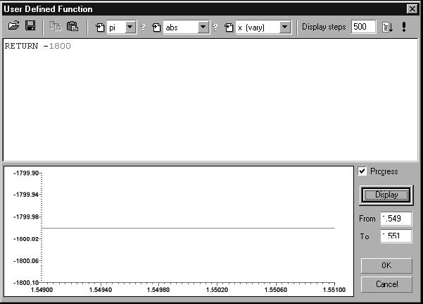
| 9 | In this screen, set the dispersion to -1800 ps/nm for all wavelengths, as seen above. |
| 10 | Click OK. |
| 11 | Click the Causality button to see the impulse response of the specified spectrum. |

| 12 | Click Close. |
Step 2
| 1 | Click Start in the Inverse Problem Solver dialog box to start the layer peeling algorithm.. |
| 2 | Select the Delay tab. |
| 3 | Select the red and light blue curves to show the transmitted and reflected delays. The dark blue curve shows the target delay. |
| 4 | Click in the graph window and go to Tools > Group Delay |

- The window displays the reconstructed group delay with a second order fitting.
The dispersion is reported in the Results frame as -1773.79 ps/nm, in close
agreement with the desired response.