
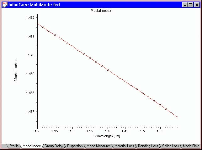
“Joints” command
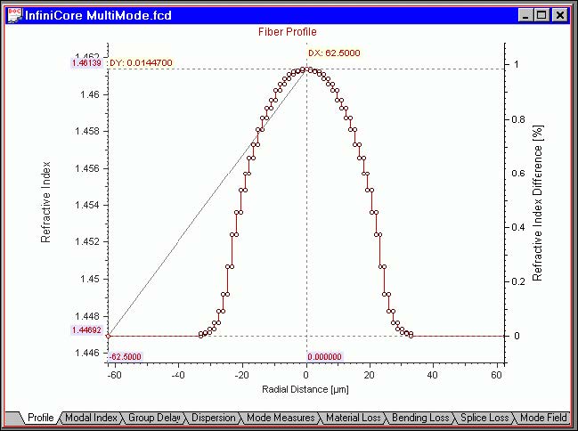
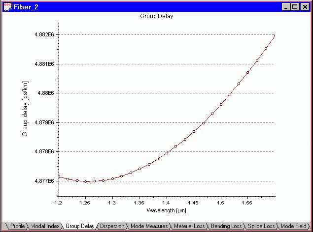
The “Joints” command activates the display of data points in the active output view.
The data points are marked as small circles.
This command can be accessed from:
- Graph Tools toolbar
- Floating menu (right mouse button on a graph)
“Zoom XY” command
The “Zoom XY” command serves to expand horizontally and vertically a part of the
active output view.
This command can be accessed from:
- Graph Tools toolbar
- Floating menu (right mouse button on a graph)
To use this command:
| Step | Action |
| 1 | Select “Zoom XY” from the Graph Tools toolbar or from the floating graph menu. |
| 2 | Now, with the left mouse button, click-and-drag a horizontal and vertical region to be expanded to a full graph. For example, before you release the left mouse button, your “Material Loss” view should look something like this: |
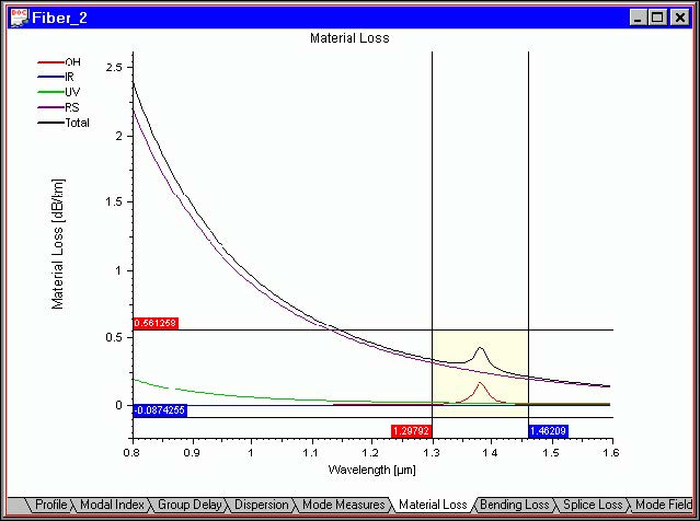
After you release the left mouse button, the selected horizontal and vertical region is
expanded to the full view.
To revert to the original graph, select “Zoom Off” from the floating menu or ”Graph
Tools“ toolbar.
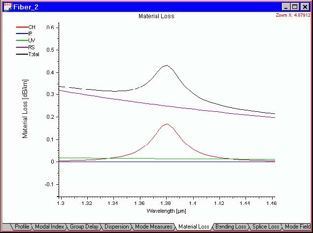
“Zoom X” command
The “Zoom X” command works identically with “Zoom XY” command except that it
expands the view only in horizontal direction.
“Zoom Off” command
The “Zoom Off” command turns off the current expansion in graph view and returns
the graph settings to the default scale.
This command can be accessed from:
- Graph Tools toolbar
- Floating menu (right mouse button on a graph)
“Measure” distance command
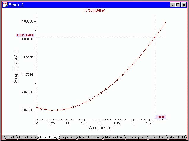
The “Measure” distance command activates the display of two crossing-line sets in
the active output view. The horizontal and vertical crossing lines show two data points on a curve along with a display of their XY coordinates and distances. The displayed
coordinates refer to the curve data points.
This command can be accessed from:
- Graph Tools toolbar
- Floating menu (right mouse button on a graph)
To use this command:
| Step | Action |
| 1 | Select “Measure” from the “Graph Tools” toolbar or from the floating graph menu. |
| 2 | Click the curve with the left mouse button. The nearest data point is displayed as a small circle with a set of XY lines passing through it. The point coordinates are displayed along the XY lines. |
| 3 | Move the cursor along the curve. During that move, the point closest to the cursor will be displayed as small circle with a second set of XY lines passing through it. The second set of lines displays the second point coordinates as well as the XY distances from the first point. |
The “Measure” distance tool works well with the “Joints” command active.
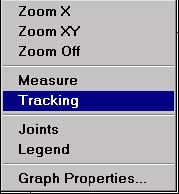
“Tracking” command
The “Tracking” command activates the display of a crossing-line set in the active
output view. The horizontal and vertical crossing lines show data points on a curve
along with a display of their XY coordinates.
This command can be accessed from:
- Graph Tools toolbar
- Floating menu (right mouse button on a graph)
To use this command:
| Step | Action |
| 1 | Select “Tracking” from the “Graph Tools” toolbar or from the floating graph menu. |
| 2 | Click the curve with the left mouse button. The nearest data point is displayed as a small circle with a set of XY lines passing through it. The coordinates of the point are displayed along the XY lines. |
Note: The simplest way to use this command is to click-and-drag on the
graph using only the left mouse button. In that case you do not need to use
the Graph Tools toolbar nor the floating menu.
The “Tracking” tool works well with the “Joints” command active.
“Legend” command
The “Legend” command toggles the display of the curves legends in the output
“Views” window.
This command can be accessed from:
- Graph Tools toolbar
- Floating menu (right mouse button on a graph)
For example the Material Loss view legend looks like this:
You can drag the legend around the graph to position it in a convenient spot.
“Grid X” command
The “Grid X” command toggles the display of the vertical grid in the active output
Views window.
This command can be accessed from:
- Graph Tools toolbar
When you select the “Grid X” command, your display will have a set of vertical lines.
The grid lines correspond to the coordinate-labeled points on the X-axis.
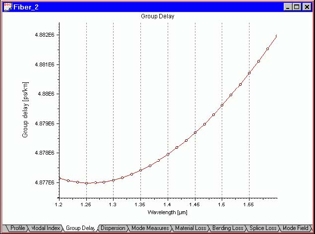
You can combine the “Grid X” and “Grid Y” command to obtain a rectangular XY grid
on the display.

“Grid Y” command
The “Grid Y” command toggles the display of the vertical grid in the active output
Views window.
This command can be accessed from:
- Graph Tools toolbar
When you select the “Grid Y” command, your display will have a set of horizontal
lines. The grid lines correspond to the coordinate-labeled points on the Y-axis.
You can combine the “Grid X” and “Grid Y” command to obtain a rectangular XY grid
on the display.
“X Cut” command
The “X Cut” can be used in the “Mode Field” output view. It allows you to track an X
cross-section of the XY mode field. By default it is turned on.
This command can be accessed from:
- Graph Tools toolbar
To use this command
| Step | Action |
| 1 | Select “X Cut” from the Graph Tools toolbar. |
| 2 | In the “Mode Field” view, click-and-drag the X-section position along the Yaxis. Along with the X-section green horizontal line , the program displays the X-section field curve. |
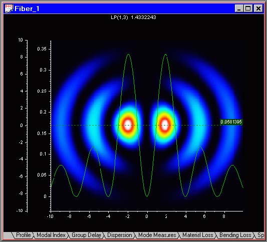
On the graph, there are two vertical scales: one corresponding to the Y-dimension of
the fiber, and the other one corresponding to the mode field section.
“Y Cut” command
The “Y Cut” can be used in the Mode Field output view. It allows you to track a Y
cross-section of the XY mode field. By default it is turned on.
This command can be accessed from:
- Graph Tools toolbar
To use this command:
| Step | Action |
| 1 | Select “Y Cut” from the “Graph Tools” toolbar. |
| 2 | In the “Mode Field” view, click-and-drag the Y-section position along the Xaxis. Along with the Y-section red vertical line, the program displays the Ysection field curve. |
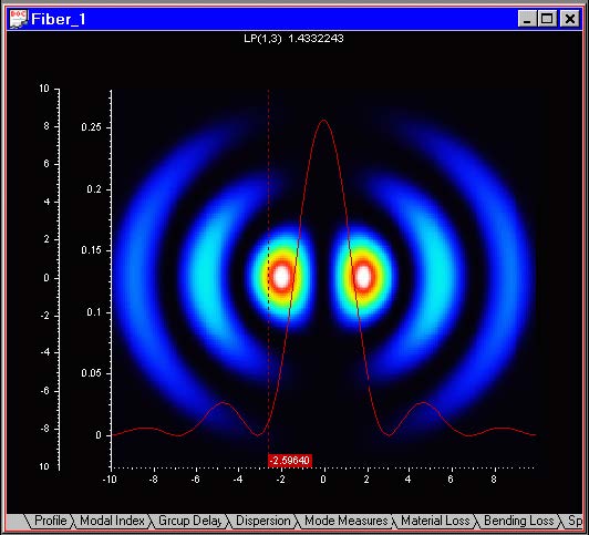
On the graph, there are two vertical scales: one corresponding to the Y-dimension of
the fiber, and the other one corresponding to the mode field section.