
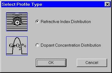
Select Profile Type dialog box
Currently OptiFiber supports two types of profiles
- Refractive index profile
- Dopant concentration profile
The “Select Profile Type” dialog box offers a choice between them. After that it popsup
the “Fiber Profile” dialog box.
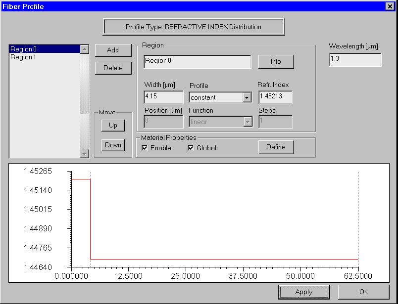
 Fiber Profile dialog box
The “Fiber Profile” dialog box helps you design the refractive index profile of the fiber.
To access this dialog box do one of the following:
- Select “Profile” on the “Fiber” menu, or
- Click the “Fiber Profile” icon in the “Navigator” pane
When the profile type is “Refractive index” the dialog box looks as shown:
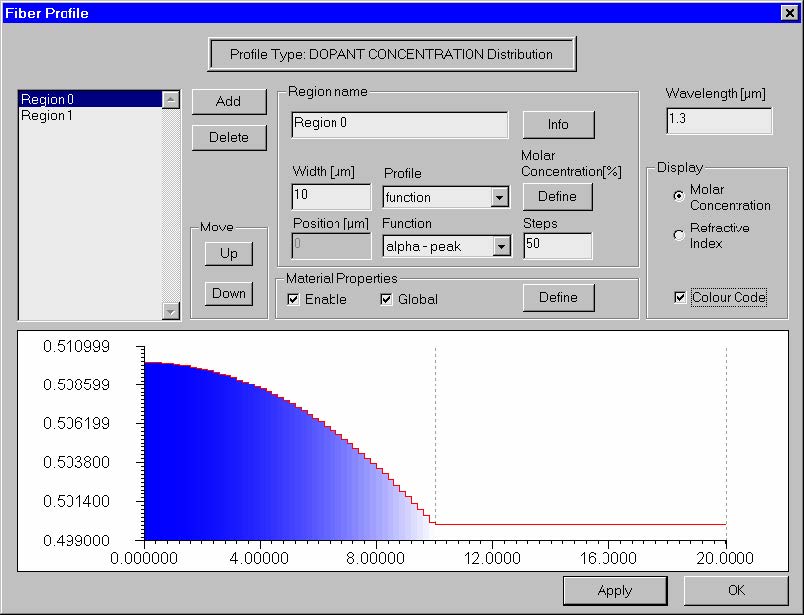
 When the profile type is “Dopant concentration” the dialog box look as shown:
The elements and controls of the “Fiber Profile” dialog box are described below.
List of Regions
Shows the radial refr. index or concentration regions by their names.
Add
Adds a region to the list.
Delete
Deletes the selected region from the list.
Up
Moves the selected region one position up the list.
Down
Moves the selected region one position down the list.
Region Name
Edits and changes the name of the selected region.
Info
Opens the “Region Info” display box, where you can see the region refractive index
with its start and end values. This option is particularly useful when dealing with user
defined regions, where the start and end index values may not be obvious.
Width
Enter the width of the selected region in microns.
Profile
Select one of the following options for the index profile within the current region:
- Constant – Constant value of the refractive index.
- Function – Functional dependence of the index, where the function is selected
from the list in the “Function” option (see “Function” below for the list of available
functions). - User Function – Functional dependence of the index, where the function is defined
or programmed using the powerful Script Language environment.
Refr. Index / Molar Concentration [%]
Depending on the select profile type this edit control is interpreted in two different
ways:
Refr. Index
Depending on the “Profile” option, you have different options for the “Refr. Index”
entry:
- Numerical data entry box – Present when the “Constant” profile option was
selected. Enter the refractive index value for the selected region. - “Define” button – Present when the “Function” or “User Function” option was
selected. Press the “Define” button to specify the function. For the “Function”
profile option, a dialog box related to one of the predefined functions appears. For
the “User Function” profile option, pressing the “Define” button launches the “User
Defined Function” script programming environment.
Molar Concentration [%]
Similar to the previous case, however all numerical values are interpreted as molar
concentration percentages, instead of refractive indices.
Position
Shows the region radial position in microns. The region position is measured from the
fiber center to the beginning of the region.
Function
This option is enabled when the “Function” profile option is selected. The program
provides the following predefined index functions:
- Linear
- Parabolic
- Gaussian
- Exponential
- Alpha-peak
- Alpha-dip
The notation convention for these functions is described in the “Technical
Background”, section “Refractive Index of Fibers”. Usually, the functions’ argument is
the radial local distance that is zero at the beginning of the region and is equal to the
“Width” value at the end of the region.
Steps
Enter the number of steps for discretization of the index profile function. The OptiFiber
mode solver requires the step-like discretization of smooth index profiles. Increasing
the number of steps provides better mode solving accuracy, however, at the expense
of calculation time.
Enable
Enable the material dispersion model for the current region. To access the model
definition press the “Define” button in the “Material Properties“ section of the dialog
box (also see “Material Properties” dialog box).
Global
Assign the global material dispersion model to the current region. The global model
assumes that a fiber is formed by doping the host material with one dopant that rises
the refractive index and another dopant that lowers the index (see “Material
Properties” dialog box).
Define
Opens the “Material Properties” dialog box, where you can assign material dispersion
model based on the Sellmeier coefficients library or on your custom model, as well as
nonlinear refractive index of the material.
Wavelength
The wavelength entered here is considered the measurement wavelength, that is, the
wavelength at which the current profile is exact. At other wavelength values used in
the program, for example when scanning over a spectral range, the profile shape is
adjusted accordingly based on the material dispersion model.
Apply
Apply the changes made in the dialog box.
Display
This group of controls allows to show the profile in one of the two alternative ways: 1)
as a refractive index profile, or 2) as dopant concentration profile. A check-box that
switches the color-coding of the profile on/off is also available.
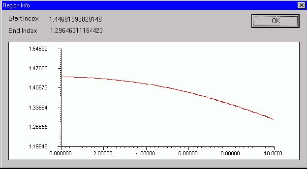
Info dialog box
The “Info” dialog box displays the selected index profile region. You can see the
region refractive index with its start and end values. This option is particularly useful
when dealing with user defined regions, where, due to the functional dependence, the
start and end index values may not be obvious.
To access this dialog box, do the following steps:
| Step | Action |
| 1 | Open the “Fiber Profile” dialog box. |
| 2 | Click the “Info” button. |
 Material Properties dialog box
The “Material Properties” dialog box looks and functions differently in dependence if
the type of profile is “Refractive Index” or “Dopant Concentration”.
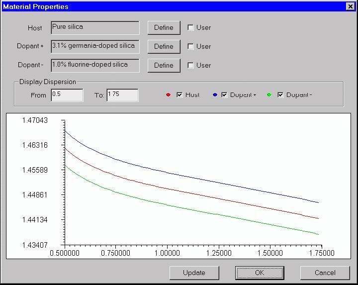
Material Properties dialog box (Profile type is “Refractive Index” )
The “Material Properties” allows the user to specify the Sellmeier and nonlinear
coefficients of the fiber material. It also displays the material refr. index as a function
of wavelength. For the dispersion model it is assumed that the fiber profile consists of
regions with only the host material and doped regions. One of the dopants rises the
refractive index, while the other dopant lowers it.
To access this dialog box, do the following steps:
| Step | Action |
| 1 | Open the “Fiber Profile” dialog box. |
| 2 | Select “Enable” in the “Material Properties” section. |
| 3 | Press the “Define” button in the “Material Properties” section. |
 The elements and controls of the “Material Properties” dialog box options are
described below.
Host
Shows the name of the fiber host material. Press “Define” to specify the material and
its dispersion model. When the “User” option is cleared, the “Define” button activates
the “Parameters of Material” dialog box. When the “User” option is checked, the
“Define” button launches the “User Defined Function” script programming
environment (see the Script Language section of the documentation).
Dopant +
Shows the name of the fiber material that has higher index due to an index-rising
dopant. The “Define” button and the “User” option work the same way as for the “Host”
option.
Dopant –
Shows the name of the fiber material that has lower index due to an index-decreasing
dopant. The “Define” button and the “User” option work the same way as for the Host
option.
Update
Update the dispersion display after recent changes.
Display From
Enter the minimum wavelength for the dispersion display.
Display To
Enter the maximum wavelength for the dispersion display.
Host, Dopant + and Dopant – check boxes
Serve to switch on /off the display of the respective curves
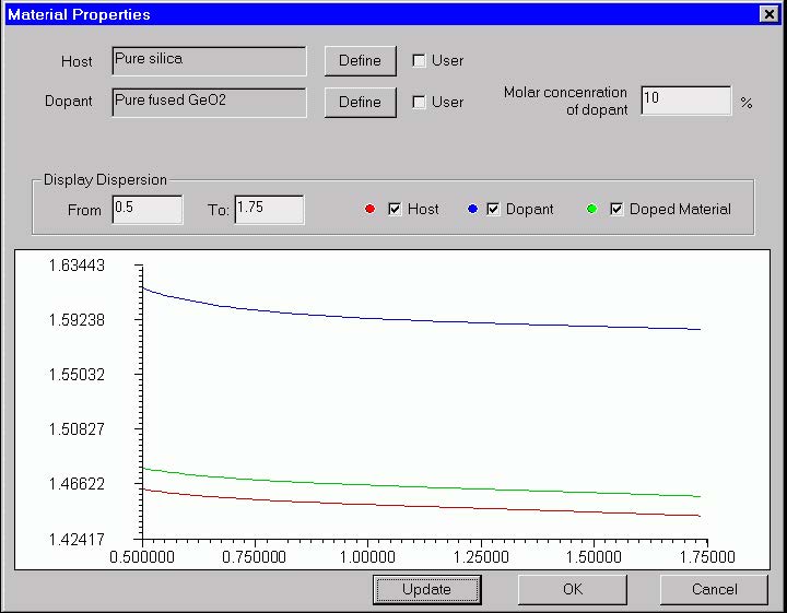
Material Properties dialog box (Profile type is “Dopant Concentration” )
The “Material Properties” allows the user to specify the chemical composition,
Sellmeier and nonlinear coefficients of the fiber material. It also displays the material
refractive indices of the pure host material, the dopant and the doped material as a
function of wavelength.
To access this dialog box, do the following steps:
| Step | Action |
| 1 | Open the “Fiber Profile” dialog box. |
| 2 | Select “Enable” in the “Material Properties” section. |
| 3 | Press the “Define” button in the “Material Properties” section. |
 The elements and controls of the “Material Properties” dialog box options are
described below.
Host
Shows the name of the fiber host material. Press “Define” to specify the material and
its dispersion model. When the “User” option is cleared, the “Define” button activates
the “Parameters of Material” dialog box. When the “User” option is checked, the
“Define” button launches the “User Defined Function” script programming
environment (see the Script Language section of the documentation).
Dopant
Shows the name of the material doping the host. The “Define” button and the “User”
option work the same way as for the “Host” option.
Molar Concentration of Dopant
Enter the molar concentration of the doping material in [%].
Update
Update the dispersion display after recent changes.
Display From
Enter the minimum wavelength for the dispersion display.
Display To
Enter the maximum wavelength for the dispersion display.
Host, Dopant and Doped Material
Serve to switch on /off the display of the respective curves
Parameters of Material dialog box
The “Parameters of Material” dialog box allows you to specify:
- The material dispersion model based on the Sellmeier theory. OptiFiber uses six
Sellmeier coefficients, three wavelengths and three amplitudes, to define the
dispersion curve. - The nonlinear coefficient of the material
- The molar concentration of dopant in case the profile type is ”dopant
concentration”.
To access this dialog box, do the following steps:
| Step | Action |
| 1 | Open the “Fiber Profile” dialog box. |
| 2 | Select “Enable” in the “Material Properties” section. |
| 3 | Press the “Define” button in the “Material Properties” section. The “Material Properties” dialog box opens. |
| 4 | In it press the “Define” button for formulate the material model of the host or the dopants. |
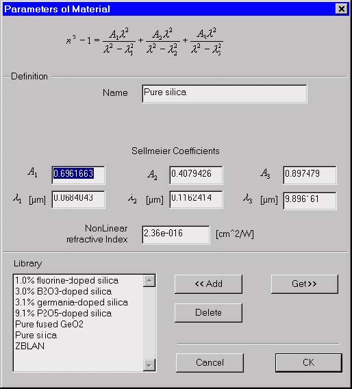 Sellmeier Formula
The Sellmeier formula is displayed for reference. The formula reads:
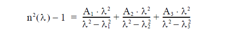
where n is the wavelength-depended refractive index, A1, A2 and A3 are the
Sellmeier amplitudes, and λ1, λ2, λ3 are the Sellmeier resonance wavelengths.
The elements and controls of “Parameters of Material” dialog box are described
below.
Name
Enter the name of the material. If you select the material from the Library list (see Get
below) then the name appears automatically.
A1, A2, A3
Enter the amplitude Sellmeier coefficients.
λ1, λ2, λ3
Enter the wavelength Sellmeier coefficients.
NonLinear Refractive Index
The nonlinear refractive index of the bulk material, as defined for example in [G.
Agrawal, 1995].
Add
If you entered new material along with its Sellmeier coefficients, you can add it to a
data base library by pressing the Add button. Using this feature the user can build rich
user-defined material libraries.
Delete
Delete the selected material from the library.
Get
Get the material from the Library list. The library materials are stored in a data base.
OptiFiber provides some of the known materials along with the Sellmeier coefficients.
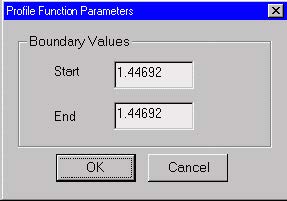
Profile Function Parameters dialog box
The “Profile Function Parameters” dialog box allows you to define the relevant
parameters of the profile function in the current region.
It covers the following types of function profiles (see also the “Refractive Index of
Fibers” section in the “Technical Background”):
- Linear index profile:
- Exponential index profile:
To access this dialog box, do the following steps:
| Step | Action |
| 1 | Open the “Fiber Profile” dialog box. |
| 2 | Select the region profile as “Function”. |
| 3 | In the “Function” list, select Linear, Parabolic, or Exponential. |
| 4 | Press the “Define” button. |
The elements and controls of “Profile Function Parameters” dialog box are described
below.
Start
Enter the start value of the refractive index or the concentration at the beginning of
the region.
End
Enter the end value of the refractive index or the concentration at the end of the
region.
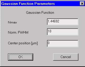
Gaussian Function Parameters dialog box
The “Gaussian Function Parameters” dialog box allows you to specify the relevant
parameters when the profile function in the current region is Gaussian (see also the “Refractive Index of Fibers” section in the “Technical Background”).
To access this dialog box, do the following steps:
| Step | Action |
| 1 | Open the “Fiber Profile” dialog box. |
| 2 | Select the region profile as “Function”. |
| 3 | On the “Function” list, select “Gaussian”. |
| 4 | Press the “Define” button. |
 The elements and controls of “Gaussian Function Parameters” dialog box options are
described below.
Nmax
Enter the maximum value of the refractive index described by the Gaussian function.
Norm. FWHM
Enter the normalized Full Width at Half Maximum (FWHM) of the Gaussian function.
Center Position
Enter the peak position of the Gaussion function. The position is measured from the
beginning of the current region.
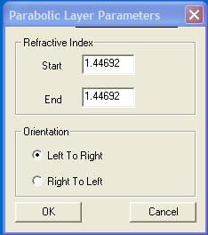
Parabolic Layer Parameters
The Parabolic Layer Parameters dialog box specifies relevant parameters for function
layers of parabolic type. See the Technical Background for the formula defining the
parabolic layer. To access this box, perform the following steps
- Open the Fiber Profile dialog box
- Select the Region profile as Function
- On the function list, select Parabolic
- Press the Define button
 The elements of the Parabolic Layer Parameters dialog box are listed below
Orientation – indicates whether the curve will start at the left and go the right side of
the layer (the default), or if the direction is to go the other way. In the default position,
the extremum of the parabola is on the left, the other orientation will put the extremum
on the right side.
Start – enter the refractive index of the layer at the start (left side in Left to Right
orientation)
End – enter the refractive index of the layer at the end (right side in Left to Right
orientation)
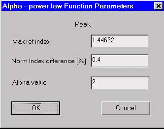
Alpha Power Law Function Parameters dialog box
The “Alpha Power Law Function Parameters” dialog box allows you to specify the
relevant parameters when the profile function in the current region is of the following
types (see also the “Refractive Index of Fibers” section in the “Technical
Background”):
- Alpha –peak index profile:
- Alpha –dip index profile:
 To access this dialog box, do the following steps:
| Step | Action |
| 1 | Open the “Fiber Profile” dialog box. |
| 2 | Select the region profile as “Function”. |
| 3 | On the “Function” list, select “Alpha-Power Peak” or “Alpha-Power Dip”. |
| 4 | Press the “Define” button. |
The elements and controls of “Alpha Power Law Function Parameters” dialog box
options are described below.
Max Ref Index
Enter the maximum value of the refractive index described by the Alpha-Power
function.
Norm Index Difference %
Enter the normalized index difference of the Alpha Power function.
Alpha Value
Enter the alpha power coefficient value.
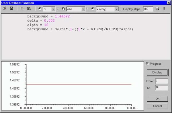
User Defined Function dialog box
The “User Defined Function” dialog box allows you to define unusual, specific
functional dependencies of the profile or the material dispersion model. The user
defined function can be almost anything that conforms to the rules of the Script
Language programming.
 Working with user defined functions
Since User Defined Functions are important for your work, you may want to have a
look at the following example:
Let’s say that you want to use a user-defined function to define a fiber profile region.
To do this, open the “Fiber Profile” dialog box and select the index region where you
want the user function to apply. Next, select the “User Function” profile option for that
region and press “Define” under the “”Refr. Index” or “Molar Concentration” heading
(depending on profile type) to open the “User Defined Function” dialog box. It is split
into two: the editing area and the display area.
The Editing Area
You define the function in the editing area. For your convenience, the editing area is
a simplified programming editor. To define a function, you type the function formula
or simply select a function from a combo box (see below: Using Combo Boxes). In the
formula, you can use numbers, constants, variables, and other functions. Standard
mathematical operators are supported. The program keeps a list of mathematical
constants, design (global) variables, and mathematical functions.
In general, the User Defined function has one independent variable, called x.
The Display Area
The graph of the function is shown in the display area.
Working in the Editing Area
Let’s assume that you need the profile of the zero-order Bessel function, J0(x/s),
where s=4. All you have to do is type the following two lines in the User Function
Definition editing area:
s=4
bessj0(x/s)
Exploring the User Defined Function program editor
As mentioned above, the editing area is a simplified programming editor. You can
write your own functions and also test and debug the program. The format of the
language is very close to BASIC. For more information, see the Script Language
documentation.
Using Combo boxes
There are three combo boxes. Each of them contains an icon and a list of options:
![]()
The icon on the left side of any combo box is for inserting a selected item into the text
(at the cursor position). The list of options in the first combo box contains all constants,
in the second one all functions, and in the last one the actual global variables. The
question marks on the right side of the first and the second combo box will give you a
short help about a constant or a function. (Usually a value for a constant and syntax
for a function.)
Using the Display Steps box
You use the “Display Steps” box for testing. In this box, you type the number of points
you will calculate when you press the Display button in the display area. The number
you type in this box is not the number of points this function will calculate in a real
calculation. To do the calculation, just press the “OK” button in the display area.
Running the Program and Debugging
![]()
The User Defined Function program editor allows you to Debug and Run (Display) the
program.
Run
The “!” button, has exactly the same function as the Display button. It is put on the
Toolbar for convenience.
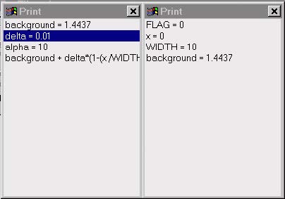
Debug
You can not only run your program but also debug it. If the function is not simple, i.e.
it may have an IF – THEN structure for example, and gives you bad results, you can
easily debug your program by pressing the Debug button and following the prompts.
In that case, you will see two new windows. The first one contains the Source Code
and shows you where you are in debugging; the second one contains a list of all
global (system defined) and local (defined by you) variables.
Exploring the Display Area
In the display area, you see the actual graph. You can also define the variable range
of x in the “From” and “To” boxes.
The Progress check box
![]() If you enable the “Progress” check box, you will be able to see the Progress Bar while
If you enable the “Progress” check box, you will be able to see the Progress Bar while
the program is running. To perform this, you have to enable the Progress check box
and press the Display button. You may want to disable the Progress check box if you
are using some output windows or FOR – NEXT loops that will give you many
Progress/Message bars.
The Load and Save buttons
![]() You can load or save any functions to disk as a separate text so that you can build
You can load or save any functions to disk as a separate text so that you can build
your own library of new functions.
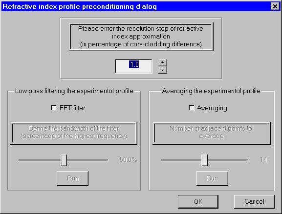
Refractive index profile preconditioning dialog
This dialog box controls the process of importing experimental refractive index data
scanned with the NR- 9200 Optical Fiber Analyzer from EXFO Inc.
 The elements and controls of “Profile Function Parameters” dialog box are described
below.
Resolution step
This is the minimal refractive index difference between two adjacent experimental
points that are to be considered belonging to different refr. index regions in OptiFiber.
It is entered in percentage of the core/cladding difference of the current profile. By
choosing larger step the user can reduce the number of fiber layers at the expense of
lower refractive index resolution. As the number of experimental points could be quite
large (thousands) the choice of the step is a matter of a reasonable compromise
between accuracy and computer load. A step value of 0 (the default value) means that
every experimental point will be considered a separate layer/region in OptiFiber.
Low-pass FFT filtering / Averaging
These two features serve to smooth the experimental profiles and remove ripples,
small spurious peaks due to vibrations, etc. The Filtering/Averaging operations are
optional, not obligatory and can be skipped. Therefore the respective areas of the
dialog are initially grayed. However, in such cases the number of interpreted fiber
layers and thus the computational effort are increased considerably. If the user opts
to smooth the profile, he has to activate the respective controls by checking the checkboxes “FFT Filter On” and/or “Averaging On”.