To add a new profile to the Profile Designer, perform the following procedure.
| Step | Action |
| 1 | Double-click on the waveguide in the layout window.
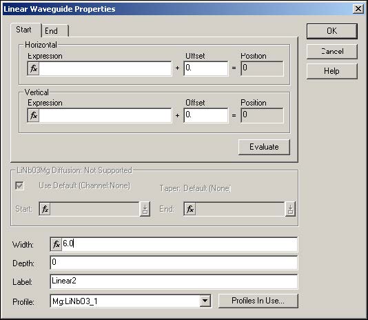
The Linear Waveguide Properties dialog box appears. |
| 2 | Click Profiles in Use.
The Profile Designer opens. |
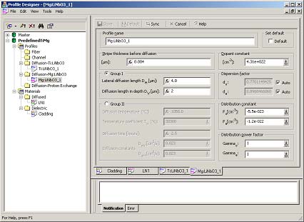
| 3 | Right-click on Diffusion profile Mg:LiNbO3 and create a new profile: Name: Mg:LiNbO3_1
Stripe thickness before diffusion: 0.004 Diffusion length in depth: 2 Lateral diffusion length: 4.0 |
| 4 | Return to the layout window. |
Creating the top linear waveguide
To draw a new linear waveguide of the same width (6 μm) on top of the Ti diffused one, perform the following procedure.
| Step | Action |
| 1 | Copy (Ctrl-C) and paste (Ctrl-V) the original waveguide in the layout
window. A second linear waveguide appears in the layout window on top of the original one. |
| 2 | Double-click on the new waveguide to open the waveguide properties dialog box. |
| 3 | Change the Profile in Use to Mg:LiNbO3_1 (see Figure 11). |
Figure 10: Linear Waveguide Properties dialog box—new waveguide
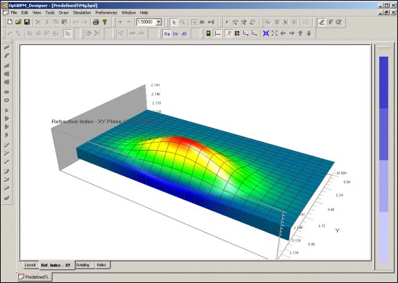
Note: Since the diffused processes are additive, the top waveguide is not going to overwrite the bottom waveguide but both processes will contribute to the final refractive index distribution. You can check the index distribution in the designer by going to the Ref.Index tab (see Figure 12).
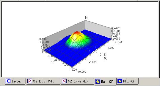
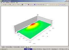
You can now run the 3D simulation (see Figure 13 and Figure 14 for 3D results).
Figure 11: Mg:LiNb03_1 profile
Figure 12: Refractive Index 3D view
In diffused waveguides, the refractive index is small. To view the diffusion, set the scale manually:
| Step | Action |
| 1 | Right-click on the graph. |
| 2 | Select Data Clamping Settings. |
| 3 | Unselect the Auto scale. |
| 4 | Enter Min = 2.137 and Max = 2.142 |
| 5 | Click Apply.
Note: Auto scale will stay off until you turn it back on, so don’t forget to turn Auto scale back on when viewing other data. |
Figure 13: Ex – XY results 3D
Figure 14: RIdx – XY results 3D


