
Design without amplification
In this example, our goal is to design a basic transparent ring network without amplification and discover the power related issues.
Metro networks using ring topology are expected to have more dynamic traffic patterns compared to most long-haul networks. They are also expected to have optically transparent nodes with a minimum number of regenerators. Therefore, we need to consider all the optical power variations that may result from several factors:
- wavelength dependent loss in fibers
- wavelength dependent gain in amplifiers
- channel to channel insertion loss variation in the multiplexers/demultiplexers
These optical degradations accumulate along the links until the optical termination is reached. Due to dynamic nature of the network, only proper dynamic power level management can reduce them.
Optical Add/Drop Multiplexers (OADMs) introduce insertion loss that contains two parts: deterministic and random. In fact, loss varies with the wavelength. The loss of fiber depends on fiber type and wavelength. Variation of optical switch types and different path lengths in the network will result in a random loss, which is difficult to predict.
There are several limiting factors in terms of power in optical networks, including:
- nonlinear effects
- receiver sensitivity
- losses in the fiber, OADMs, OXCs
We will consider all these effects in our design and simulations.
Typical loss, transmitter power, and receiver sensitivity values are given in Table 1 and Table 2.
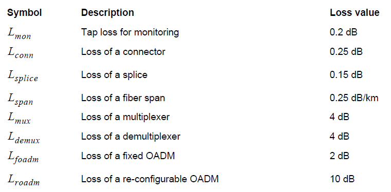
Table 1: Typical losses for components used in metro links
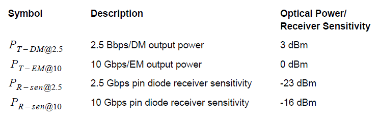
Table 2: Typical values for transmitter and receiver
Total allowable loss from transmitter to receiver depends on the transmitted power and receiver sensitivity. As shown in Table 2, receiver sensitivity is also a function of bit rate. The allowable loss is given by Lallowable = PT = PR-sens. Assuming two splices and six connectors, total loss at each node is given by Lnode = 2Lsplice + 6Lconn + Lfoadm.
Let us consider a typical WDM metro ring at 2.5 Gbps, with a 200 km circumference and four intermediate fixed OADMs, as shown in Figure 1. In this network, node 1 and 4 communicate on channel 1, whereas node 2 and 3 communicate on channel 2. The project is found in the Optical power level management in metro networks_Linear.osd and Optical power level management in metro networks_NA.osd files. These are two versions of the same project, one with linear fibers and one with nonlinear fibers. We will first investigate the system performance without fiber nonlinearities. Then we will enable fiber nonlinearities to see if a design without considering nonlinearities really works in real life.

Figure 1: A basic optical ring network with four node and two channel
Without any inline amplification, the allowable loss by using direct modulated source is Lallowable = 3-(-23) = 26 dB. Node (including two splices and six connectors) and span losses are Lnode = 2×0.15+6×0.25+6×0.25+2=3.8 dB and Lspan50km = 13.5 dB. Therefore total loss will be 3x(13.5+3.8)=51.9dB.
Comparing the allowable loss and total loss in the network shows that it is not a good idea to make a design without amplification. Of course, increasing power is another option, but nonlinear effects may become important impairments at high powers. In this case, allowing 3 dB system margin, the required launch power will be the following:
51.9 +3-23=31.9 dBm/channel
Now let us try to estimate the threshold values for fiber nonlinearities.
Self-Phase Modulation
The effect of SPM is to chirp the pulse and broaden its spectrum. As a rough design guideline, SPM effects are negligible when P0 < α / y where y = n2ω0/cAeff [1/(Wkm)] is the nonlinearity coefficient, P0 is the peak power, and α is the loss parameter.
For the fiber, we used y ≈ 1.5w-1km-1. Therefore, SPM effects can be negligible when the total peak power is below 180 mW or 19 dBm average power.
Cross-Phase Modulation
When two or more pulses of different wavelengths propagate simultaneously inside fibers, their optical phases are affected not only by SPM but also by XPM. Fiber dispersion converts phase variations into amplitude fluctuations. XPM induced phase shift should not affect the system performance if the GVD effects are negligible. As a rough estimate, the channel power is restricted with Pch < α /[y(2Nch-1, where Nch is the number of channels.
For a two channel system, limiting power is around 60 mW (14.5 dBm per channel). Separation between channels also affects the XPM. An increase in the separation will decrease the penalty which originates from XPM.
Four-Wave Mixing
FWM is the major source of nonlinear cross-talk for WDM communication systems. It can be understood from the fact that beating between two signals generates harmonics at difference frequencies. If the channels are equally spaced new frequencies coincide with the existing channel frequencies. This may lead to nonlinear cross-talk between channels. When the channels are not equally spaces, most FWM components fall in between the channels and add to overall noise. FWM efficiency depends on signal power, channel spacing, and dispersion.
If the GVD of the fiber is relatively high |β2| > 5ps2 / km, the FWM efficiency factor almost vanishes for a typical channel spacing of 50 GHz or more. If the channel is close to the zero dispersion wavelength of the fiber, considerably high power can be transferred to FWM components. To reduce the effect of FWM on system performance, you can use either uneven channel spacing or a dispersion-management technique.
Stimulated Raman Scattering
Because of SRS, short wavelength channels act as pumps for longer wavelength channels. In a WDM system, the SRS impairs the system performance because energy is transferred from the short-wavelength to the long-wavelength channels. The Raman threshold for a single channel system is given by:
![]()
and it is approximately equal to 1 / α for long fibers. In fact, it is a function of the number of the channels and channel power. For a single channel system it is around 500 mW near 1.55 micrometer if gR = 1×10-13m/W. For a 20 channel system Pth exceeds 10 mW whereas it is around 1 mW for a 70 channel system. It has little impact on system performance.
Stimulated Brillouin Scattering
SRS is the result of the interaction of light with acoustic waves in fiber which scatters power backward. Back scattered light is downshifted in frequency from the original signal frequency. Threshold level depends on:
- source line-width
- effective core area
- effective fiber length
Typical value for gB is approximately 5×10-11m/W. The threshold value also depends on modulation format and duration of pulse. Some values for threshold power are given below:
- 9 dBm for CW light
- 12 dBm for externally modulated transmitter
- >18 dBm for externally modulated transmitter with source wavelength dither
Generally speaking, SBS has little effect on system performance.
Figure 2 shows the Q factor for channel 1 at the receiver end versus received average power, when no in-line amplifier is used and non-linearities of the fibers are disabled. To obtain this figure, we have used directly modulated sources with 3 dBm output power. We have inserted a power amplifier after Node 1 to adjust the signal power. Thermal noises of the receivers are adjusted to obtain -2.5 Gbps sensitivity at 2.5 Gbps. When we enable the non-linearity, the eye is always closed.

Figure 2: Q factor versus received average power at node 4 when no amplifier is used and fiber non-linearity is disabled
To investigate the effect of non-linearity, we disabled the thermal noise of the PIN (which is the dominant noise in this design) and repeated the simulation. The results are shown in Figure 3. This figure shows that after about 14 dBm launch power (as predicted), non-linearity becomes an issue and Q factor starts to decay. From these figures, we can conclude that the limiting factor below the 18 dBm region is mainly thermal noise, whereas above 14 dBm, it is non-linearity. Therefore, non-linearity is an important factor in the design of transparent optical metro networks without amplification.

Figure 3: Q factor versus average received power at node 4 when no amplifier is used and thermal noise of the PIN is disabled
We have also seen that a simple power budgeting is not enough to design a transparent ring network. However, you need to run a whole detailed simulation to see the effects of fiber non-linearities on the system performance.
Design with Lumped Amplification
In this example, we will consider design of a transparent ring network with lumped amplification.
Metro ring networks have a more dynamic traffic pattern than most long-haul networks. In these types of configurations, we need to consider:
- all the optical power variations resulting from wavelength dependent losses in fibers
- wavelength dependent gain in amplifiers
- channel to channel insertion loss variations in multiplexers/demultiplexers
These optical degradations accumulate along the links and may increase very quickly, depending on the path followed by the wavelength. Due to dynamic nature of the network, only proper dynamic power level management can reduce them. Typical values for the loss elements can be found in “Design without amplification” on page 379.
Let us first investigate optical amplifiers.
Optical Amplifier
Gain and gain tilt of optical amplifiers changes with the input power. This can be seen in Figure 4 for EDFAs (length of the fiber is 4 m, pump power at 980 nm is 100 mW). (See gain variation of EDFAs.osd.) When the span losses of each span in the ring are different, the input power of each amplifier will be different. Depending on the path of the signal, each communication link between two nodes will experience different amplification. Furthermore, amplifier tilt can accumulate depending on the path followed. To eliminate this effect, pump control, variable attenuator at the input, or gain tilt compensating amplifier/filters can be used.

Figure 4: Value and shape of optical amplifiers
Figure 5 shows the results of two cascaded EDFAs (length of the fiber is 4 m, pump power at 980 nm is 35 mW, input power 17.3 dBm/channel or -133 dBm total power). (See gain variation of cascaded EDFAs.osd.) Here, we consider a 16.4 dB loss between amplifiers to model the total span and node loss. It is clear from this figure that tilt of the two-stage amplifier is increased. A channel near 193 THz will see a gain of approximately 14 dB after a two node pass, whereas it is approximately 12 dB for a channel at 194 THz. Therefore, this effect may be an issue for a 100 GHz separated 10 channel system, even though each channel passes through the same number of amplifiers.

Figure 5: Gain profile of one and two cascaded amplifiers
A typical WDM metro ring at 2.5 Gbps, with a 200 km circumference and four intermediate fixed OADMs, is shown in Figure 6. In this network, node 1 and 4 communicate on channel 1, whereas node 2 and 3 communicate on channel 2, as in the previous example. The project is found in the Optical power level management in metro networks lumped amplification.osd file.

Figure 6: Ring network layout with two amplifiers
Assuming a launch power of 3 dBm per channel, the amount of amplification needed in the ring is

This gain can be obtained by using two amplifiers as shown in Figure 6. In this configuration, two amplifiers with 15 dB gain are placed just before node 2 and node 4. Note that required gain is higher than the gain target value for metro EDFAs (see Table 1). Therefore, a single amplifier configuration is not practical for metro applications. Keep in mind that even though this amplifier design gives sufficient performance, scalability of this configuration will be complicated.

Table 1: Typical values for amplifiers
Figure 7 shows Q factor versus received average power for two-amplifier configurations.

Figure 7: Measured signal power and OSNR
This figure shows about -11 dBm average received power. Q factor is maximum and below 4.5. Figure 8 shows the eye diagram for this case. Figure 9, on the other hand, shows the trace of OSNR and signal power as obtained by using Trace Paths tool.

Figure 8: Eye diagram at node 4 when two amplifiers with 15 dB gain each are inserted before node 4 and node 2
Figure 9 shows the eye diagram when the gain of the two amplifiers are 25 dB each. In this case, the Q factor is 38, and OSNR is approximately 31 dB.
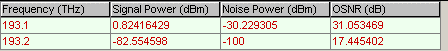

Figure 9: Trace of the OSNR and power from node 1 to node 4
These results show that this configuration provides a better system performance compared to design without amplification. Q factor that we can get from this configuration is about 4.5, due to unoptimized add/drop multiplexers and electrical filters. System performance can be further improved by carefully adjusting the transmitter and filter parameters.
Even though this configuration may give satisfactory performance for a static configuration, it will not allow addition of a new node or complex wavelength routing schemes where one signal may follow different paths depending on the routing.
Unity Gain Design
In this example we will show an alternative approach, the “unity gain” approach, in which each amplifier matches the loss of one.
In optical ring topology, we need to consider all the optical power variations resulting from
wavelength dependent loss in the fiber
wavelength dependent gain in amplifiers
channel to channel insertion loss variation in the multiplexers/demultiplexers
These optical degradations accumulate along the links and may increase very rapidly depending on the path followed by the wavelength. Due to the dynamic nature of the network, only proper dynamic power level management can reduce them. In these previous two sections, we have seen that design without amplification is not a good option, because required high power levels can trigger fiber nonlinearity.
For this approach, an amplifier with a modest gain of 17.3 dB at every node can be used. This approach is only economically feasible with a low cost-compact optical amplifier, but it is the best one considering the dynamic routing in the network.
Let us now consider a typical WDM metro ring at 2.5 Gbps with 200 km in circumference with four intermediate fixed OADMs as shown in Figure 1. In this network, node 1 and 4 communicate on channel 1 whereas node 2 and 3 communicate on channel 2, as in the previous cases. Loss of each span and node is compensated at the node following the span. The gain of each amplifier is 17.3 dB. The project is found in the Optical power level management in metro networks unity gain.osd file. This configuration is scalable, since regardless of the path followed by a certain wavelength, the power is always balanced.

Figure 1: Ring network layout with amplifier at each node
Eye diagrams of channel 1 at node 4 is shown in Figure 2, where received average power is 0 dBm. Figure 3 shows the eye diagram at node 4 when average received power is 12 dBm. Figure 4 shows Q factor versus received average signal power.

Figure 2: Eye diagram of channel 1 at node 4 when received average power is about 0 dBm and bit rate is 2.5 Gbps

Figure 3: Eye diagram of channel 1 at node 4 when received average power is about 12 dBm and bit rate is 2.5 Gbps

Figure 4: Q factor versus average received power at node 4 when bit rate is 2.5 Gbps
Figure 9 shows the trace of OSNR and signal power as obtained by using Trace Path tool. This figure shows that the signal power is balanced throughout the light path for channel 1, at 193.1 THz. Of course, this will increase the scalability of the optical metro network. Moreover, dynamic wavelength routing can be easily implemented in this type of network. Also note that this configuration is less sensitive to power changes. This is a result of balanced power throughout the network.

Figure 5: Trace of OSNR/power from node 1 to node 4 when received signal power is about 0 dBm
Considering the Non-Ideal Characteristics of EDFAs
In this example, we will consider an all optical two-ring network connected with OXCs and investigate the effects of amplifier control mode to network performance.
We will consider a two-ring system as shown in Figure 1. The project is found in the Considering nonideal characteristics of EDFA_power.osd file.

Figure 1: Two interconnected ring network layout
In this system, each ring can be used as a protection path for the other. A functional diagram of OXCs is shown in Figure 2.

Figure 2: Functional diagram of OXCs Each
Each span between nodes is made up of a single mode fiber and an EDFA (to compensate the span loss). In this project, we used Black Box EDFA models. For the sake of simplification, we have used the Directly Modulated Laser Measured model for transmitters and set chirp-related factors to zero. Therefore, we neglect any system penalty related to initial chirp on the signal.
Chirp-related issues will be discussed in the Negative Dispersion Fiber for Metro Networks tutorial. In this network, node 1 communicates with node 4 on channel 1, node 5 communicates with node 7 on channel 2, node 6 communicates with node 8 on channel 3, and node 2 communicates with node 3 on channel 4. The frequency spectrum of the channels is shown in Figure 3. Node 1 can send data following a path passing through 1, 2, OXC 1, 3, OXC 2, 4. This path requires 4 amplifications.

Figure 3: Power spectrum of the 4 channel-8 node ring network
For this example, we will presume that there is a fiber break between OXC 1 and OCX 2 or a problem at node 3, while node 1 wants to send data to node 4. Depending on the switching of OXC 1 and OXC 2, there is more than one path that the signal on channel 1 can follow. Let us assume that node 1 communicates with node 4 following the path passing through 1, 2, OXC 1, 5, 6, 7, OXC 2, 4, by using the second ring as the recovery path. This path will require 6 amplifications.
Because of the dynamic nature of the metro network, total power at the input of each amplifier will be different depending on the wavelength routing. Moreover, the gain spectrum is not flat, but tilted, so it will require some extra planning to balance the power through the network.
We first set all the amplifiers to work in power control mode and set the power on the output amplifiers to 6 dBm. Considering each ring individually, this seems to be a good choice, where the power of each channel is kept at a certain level. Interaction between the rings, on the other hand, will influence the performance of the amplifiers. This is shown in Figure 4 and Figure 5.
These two figures show the eye diagrams for the two different paths, before and after the fiber break, respectively.
 is followed")
Figure 4: Eye diagram of the signal at node 4 when the first path (node 1, node 2, OXC 1, node 3, OXC node 2, and node 4) is followed
 is followed after a fiber break")
Figure 5: Eye diagram of the signal at node 4 when the second path (node 1, node 2, OXC 1, node 5, node 6, node 7, OXC node 2, and node 4) is followed after a fiber break
This example shows that due to dynamic nature of metro network, a careful and intelligent power budget planning and control should be exercised. Several strategies can be followed to solve this problem. Let us assume that the gains of the EDFAs are flattened and stabilized with respect to input power change. To model this condition, we set the EDFAs to work in gain control mode with 17.3 dB gain. The project is found in the Considering nonideal characteristics of EDFA_gain.osd file.
Simulation results are shown in Figure 6 and Figure 7, before and after the fiber break, respectively. These figures show that we can obtain a better performance for a dynamic metro network when gain-controlled amplifiers are used. We note an extra eye closure in Figure 7. This is partly related to lower SNR at node 4 when the signal follows the protection path, since there are two extra amplifiers on this path. Moreover, there will be more non-linear interaction between channels due to extra fibers that signal passes and extra channels that increase the total power in the fiber.
The results show that gain control of amplifiers is important for metro applications, and dynamic routing can be done easily without any problem when the unity gain approach is used (see “Unity Gain Design” on page 390).
 is followed and gain-controlled amplifiers are used")
Figure 6: Eye diagram of the signal at node 4 when the first path (node 1, node 2, OXC 1, node 3, OXC node 2, and node 4) is followed and gain-controlled amplifiers are used
 after a fiber break is followed and gain-controlled amplifiers are used")
Figure 7: Eye diagram of the signal at node 4 when the second path (node 1, node 2, OXC 1, node 5, node 6, node 7, OXC node 2, and node 4) after a fiber break is followed and gain-controlled amplifiers are used
References:
[1] K. M. Sivalingam and S. Subramaniam, Optical WDM Networks: Principles and Practice, Kluwer Academic Publishers, 2001.
[2] Sidney Shiba et. al., “Optical Power Level Management in Metro Networks”, NFOEC’01, 2001.
[3] R. Ramaswami and K.N. Sivarajan, Optical Networks: A practical Perspective, Morgan Kaufmann, 1998.
[4] Tarek S. El-Bawab et. al., “Design considerations for transmission systems in optical metropolitan networks”, Opt. Fib. Tech. 63, p. 213, 2000.
[5] I. Tomkos et. al., Filter concatenation in metropolitan optical networks utilizing directly modulated lasers”, IEEE Photon. Tech. Lett. 13, p. 1023, 2001.