
OptiSystem allows the design and simulation of optical fiber amplifiers and fiber lasers.
The projects presented here are available under OptiSystem installation folder samplesOptical amplifiers.
This tutorial will describe part of the library of optical amplifiers.
There are four categories of components in the library:
EDFA
Raman
SOA
Waveguide amplifiers
The EDFA folder contains the Erbium-doped fiber model and other models to allow the simulation of EDFAs in the steady-state condition. Furthermore, the folder includes models to simulate erbium-ytterbium codoped fiber, ytterbium-doped fiber and dynamic models for the erbium and ytterbium fibers.
| Component name | Folder | Icon |
| Erbium Doped Fiber | Amplifiers Library/Optical/EDFA | |
| EDFA | Amplifiers Library/Optical/EDFA | |
| EDFA Black Box | Amplifiers Library/Optical/EDFA | |
| Optical Amplifier | Amplifiers Library/Optical/EDFA | |
| EDFA Measured | Amplifiers Library/Optical/EDFA | |
| EDF Dynamic | Amplifiers Library/Optical/EDFA | |
| EDF Dynamic Analytical | Amplifiers Library/Optical/EDFA | |
| Er-Yb Codoped Fiber | Amplifiers Library/Optical/EDFA | |
| Yb Doped Fiber | Amplifiers Library/Optical/EDFA |  |
| Yb Doped Fiber Dynamic | Amplifiers Library/Optical/EDFA |
Table 1: Doped fiber models
The second category is the Raman models. These components allow the simulation of Raman fiber amplifiers. The Raman folder includes the Raman models for steady state and dynamic conditions.
| Component name | Folder | Icon |
| Raman Amplifier – Average Power Model |
Amplifiers Library/Optical/Raman | |
| Raman Amplifier – Dynamic Model |
Amplifiers Library/Optical/Raman |
Table 2: Raman models
The tutorial will use passive components that allow the design of amplifiers and lasers. These components are spread in different folders at the OptiSystem component library and some of them are described at Table 3. These are the equivalent components to those found in OptiAmplifier.
| Component name | Folder | Icon |
| Isolator Bidirectional | Passives Library/Optical/Isolators | |
| Reflector Bidirectional | Passives Library/Optical/Reflectors | |
| Attenuator Bidirectional | Passives Library/Optical/Attenuators | |
| Pump Coupler Bidirectional | Passives Library/Optical/Couplers | |
| Coupler Bidirectional | Passives Library/Optical/Couplers | |
| Tap Bidirectional | Passives Library/Optical/Taps | |
| Circulator Bidirectional | Passives Library/Optical/Circulators | |
| Polarization Combiner Bidirectional |
Passives Library/Optical/Polarization | |
| Reflective Filter Bidirectional | Filters Library/Optical/ | |
| 3 Port Filter Bidirectional | Filters Library/Optical/ | |
| Transmission Filter Bidirectional | Filters Library/Optical/ | |
| Nx1 Mux Bidirectional | WDM Multiplexers Library/Multiplexers | |
| 2×2 Switch Bidirectional | Network Library/Optical Switches |
Table 3: Passive components
Optical Amplifiers
Global parameters
The first step when using OptiSystem is setting the global parameters.
As we already know, one of the main parameters is the time window, calculated from the bit rate and sequence length.
For the amplifier and laser design, there are other important parameters that will define the number of iterations in the simulations and introduce an initial delay in the in the simulation.
These parameters are the Iterations and Initial delay, and are available in the global parameters window (Figure 1).

Figure 1: Global parameters: Signals tab
For this tutorial we will use the default parameters, except for some global parameters.
- In the global parameters dialog box, change the parameter Bit rate to 2.5e9, Sequence length to 32, and Samples per bit to 32. The Time window parameter should be 1.28e-8 s (Figure 2).

Figure 2: Global parameters: Simulation parameters tab
System setup
After setting the global parameters, we can start adding the components to design the basic EDFA design.
From the component library, drag and drop the following component in to the layout:
- From “Default/Transmitters Library/Optical Sources”, drag and drop the “CW Laser” and the “Pump Laser” into the layout.
- From “Default/Amplifiers Library/Optical/Doped Fibers”, drag and drop the “Erbium Doped Fiber” component into the layout.
- From “Default/Passives Library/Optical/Isolators”, drag and drop two “Isolator Bidirectional” components and a “Pump Coupler Bidirectional” component into the layout.
- From “Default/Receivers Library/Photodetectors”, drag and drop a “Photodetector PIN” component into the layout.
- From “Default/Visualizers Library/Optical”, drag and drop the “Dual Port WDM Analyzer” into the layout.
The next step is to connect the components according to Figure 3. As we can see, there is one input port in the isolator opened, so to be able to run the simulation it is necessary to include an optical null in the design (Figure 3 (b)).


Figure 3: EDFA layout
Signals tab
Although all components are in the layout and correctly connected, we are not able yet to run the simulation properly.
First, because we are considering the signals propagating in both directions, we will need more than one global iteration for the results in the system to converge.
Secondly, in the first iteration there are no backward signals in the left input port of the bidirectional components, such as the isolator and pump coupler. This will make the simulation stop.
To resolve the first condition, you just have to increase the number of iterations.
To resolve the second condition, there are two possible solutions: We can enable in the Signals Tab the Initial delay parameter (Figure 4) or we can introduce in the layout the component “Optical Delay” (Figure 5).

Figure 4: Global parameters – Increasing the number of iterations and enabling Initial Delay

Figure 5: Including the “Optical Delay” components in the layout
Running the simulation
We can run this simulation for the system shown in Figure 3 and analyze the results:
- To run the simulation, you can go to the File menu and select Calculate. You can also press Control+F5 or use the calculate button in the toolbar. After you select Calculate, the calculation dialog box should appear.
- In the calculation dialog box, press the Play button. The calculation should perform without errors.
Viewing the results
To see the results, double click the Dual Port WDM Analyzer. You can see the results of each iteration by browsing in the Signal Index parameter.
Figure 6 shows the results in the WDM analyzer for the 6 iterations and initial delay.


Figure 6: Dual Port WDM Analyzer views for different iterations
Running the simulation
To compare the results in the two different designs, Figure 3 and Figure 5, we can run the same simulation for the system showed in Figure 5 and analyze the results:
- To run the simulation, you can go to the File menu and select Calculate. You can also press Control+F5 or use the calculate button in the toolbar. After you select Calculate, the calculation dialog box should appear.
- In the calculation dialog box, press the Play button. The calculation should perform without errors.
Viewing the results
To see the results, double click the Dual Port WDM Analyzer. You can see the results of each iteration by browsing in the Signal Index parameter.
Figure 7 shows the results in the WDM analyzer for the 6 iterations.


Figure 7: Dual Port WDM Analyzer views for different iterations
As we can see, the second design converges faster than the design with ‘Initial Delay’. The design from Figure 3 takes more iteration because of the ‘Initial delay’.
Viewing the gain versus wavelength
We will build the graph gain as a function of the signal wavelength.
Starting using the layout from Figure 5:
- Double-click on the CW Laser component. The component properties will appear. See Figure 8 (a).
- Change the unit of the Frequency parameter to nm.
- Select the parameter that you want put in sweep mode. In this case the parameter is Frequency. Change the mode of the Frequency parameter in the CW Laser component from Normal to Sweep. See Figure 8 (b).
- Select the Parameter Sweeps tab at the CW laser properties, or at the menu tool bar, or at the Layout menu. See Figure 9.
 Frequency parameter in Normal and (b) Sweep mode")
 Frequency parameter in Normal and (b) Sweep mode")
Figure 8: CW Laser properties (a) Frequency parameter in Normal and (b) Sweep mode
 the menu tool bar and (b) at the Layout menu")
 the menu tool bar and (b) at the Layout menu")
Figure 9: Parameter Sweeps at (a) the menu tool bar and (b) at the Layout menu
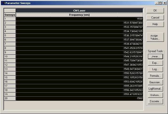
- After you click in the Parameter Sweeps tab, a window asking you to set the total number of sweep iterations will appear.
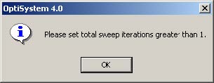
- Click on OK and the windows to enter the number of sweep iterations will appear.
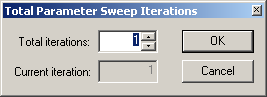
- Choose the number of sweep iterations. In this case we select 20 sweeps. After you click the OK button, the Parameter Sweeps tab will appear.
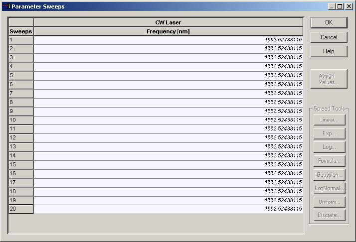
- Now we can enter the value of each sweep iteration, or we can select all the sweeps and click in one of the buttons (Linear, Exp, Log, Formula, Gaussian, etc.) to spread the values in a range. In our case we clicked in the Linear button. A new window will open to select the wavelength range in which the signal will be distributed.
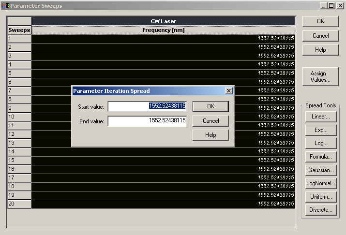
- We chose the range from 1530 nm to 1560 nm, and after we clicked on OK, the values were distributed.
Running the simulation
- To run the simulation, you can go to the File menu and select Calculate. You can also press Control+F5 or use the calculate button in the toolbar. After you select Calculate, the calculation dialog box should appear.
- In this case, we could select to simulate all sweep iterations, or choose a specific iteration and select to calculate the current iteration. For this topic, we selected to calculate all iterations. See Figure 10.
- In the calculation dialog box, press the Play button. The calculation should perform without errors.

Figure 10: Calculating all sweep iterations
Viewing the results
To see the results, double click the Dual Port WDM Analyzer. You can see the results of each iteration (global iteration) in one specific sweep iteration (wavelength) by browsing in the Signal Index parameter.
In our case, we kept the Signal Index in the last (global) iteration (5), and we can browse in the results for all (wavelengths) sweep iterations by clicking in the icons “Next Sweep Iteration” and “Previous Sweep Iteration”.
Figure 11 shows the results in the WDM analyzer for the sweep iteration number 20 and 19.
 20 and (b) 19")
 20 and (b) 19")
Building the graph Gain x Wavelength and Noise Figure x Wavelength
- The next step would be to visualize gain and noise figure for all wavelengths simulated. Therefore, we need to build graphs with the results found in the simulation.
- For this task, we will use the Report page.
- Go to the Report tab and click on it. See Figure 12.

Figure 12: View of the GUI with the system layout
- The report page will appear. After that, select the Opti2Dgraph (graph icon highlighted) and open in the report page a 2D graph. See Figure 13.

Figure 13: View of the report page
- After opening the 2D graph, go to the project browser window and open the parameter folder of the component that has the information you want. In this case we need the wavelength of the CW Laser, so we selected the Frequency parameter. See Figure 14.

Figure 14: View of the report page with the graph opened and the Frequency parameter selected
- The Frequency parameter was then dragged to the 2D graph and dropped at the X-axis. See Figure 15.

Figure 15: View of the report page with Frequency parameter being dropped at the graph
- After dropping the Frequency parameter, we have to get the next variable of the graph. So go to the Dual Port WDM Analyzer and open the Results folder.
- Choose one of the results that you want plot in your graph. In this case, we choose the Gain parameter. Now, drag and drop it in the y-axis in the graph. See Figure 16.

Figure 16: View of the report page with the Gain result being dropped at the graph
- After that, the graph Gain x Wavelength is ready. See Figure 17(a). The same procedure was used to build the graph NF x Wavelength.
 Gain x Wavelength and (b) NF x Wavelength")
 Gain x Wavelength and (b) NF x Wavelength")
Figure 17: Graphs (a) Gain x Wavelength and (b) NF x Wavelength
Optimizing the Fiber length
In addition to using the sweep iterations to analyze the amplifier characteristics (such as gain versus signal wavelength and gain versus doped fiber length), the user can use the optimization tool to find the best parameters for the amplifier design.
In this example, we will use the optimization tool to find the best doped fiber length to get the maximum signal gain.
- Load the same layout presented at Figure 5. Remember to return the Total Number of Sweep Iterations to 1 if you had changed it.
- Run the simulation. This step is necessary to setup the Dual Port WDM Analyzer for the optimization.

Figure 18: Layout of the system to be optimized
Viewing the results
After you run the system, double click in the Dual Port WDM Analyzer to see the results.
To see the results in different iterations and set the Signal Index to the last iteration, see Figure 19.
To guarantee the optimization will work correctly, you need to set the visualizer Signal Index to the last iteration.

Figure 19: Dual Port WDM Analyzer set with the results of the last iteration
Setting up the Optimization
- Go to the tools menu and click in Optimizations. See Figure 20.

Figure 20: Optimizations option at the Tools menu
- The Optimizations window will appear.
- There are two options for the optimization: the Single Parameter Optimization (SPO) and the Multiple Parameter Optimization (MPO). In our case, we want only to optimize the Fiber length as a function of the gain, so we can select the SPO and insert it on the project. For example, Figure 21 displays the calculation window and the optimization tab.

Figure 21: Optimizations tab during calculation
- When we insert the SPO optimization, the SPO Setup window will open. See Figure 22.
- In the Main tab, select the Optimization Type you want. In this case we selected to maximize the result.
- Setup the number of passes and the result tolerance.

Figure 22: SPO Setup window at the Main tab
- Go to the Parameter tab in the SPO Setup and select the parameter that you want to optimize. In this case, Length at the Erbium-doped fiber component. See Figure 23.
- After you select the parameter, specify the range of values you want to analyze. Be careful in choosing these values, they have to match the unit chosen in the Component parameter. For this case there is only one unit, meter. But in some cases, such as for power, the unit could be W, mW or dBm.

Figure 23: SPO Setup window at the Parameter tab
- In the Result tab, select the result in the Dual Port WDM Analyzer that you want to maximize (Gain). See Figure 24.
- Because we want to maximize the gain, the Target value will not be enabled.
- Click on ok in the SPO Setup.
- To run the simulation you can go to the File menu and select Calculate. See Figure 25.
- Before you press the Play button, click in the box to run all optimizations. Then, press the Play button.

Figure 24: SPO Setup window at the Result tab

Figure 25: Calculate window
During the calculation, the parameters and results of each pass will appear in the Optimization Tab. See Figure 26(a).
In the calculation output tab will appear the optimum fiber length where we got the maximum gain for the signal at 1530 nm.
 Optimization tab and (b) Calc. Output tab")
 Optimization tab and (b) Calc. Output tab")
Figure 26: (a) Optimization tab and (b) Calc. Output tab