
This lesson describes how to create a transmitter using an external modulated laser. You will become familiar with the Component Library, the Main layout, component parameters, and visualizers.
To start OptiSystem, perform the following procedure:
Starting OptiSystem

Figure 1: OptiSystem graphical user interface
Main parts of the GUI
The OptiSystem GUI contains the following main windows:
- Project layout
- Dockers
-
- Component Library
- Project Browser
- Description
- Status Bar
Project layout
The main working area where you insert components into the layout, edit components, and create connections between components (see Figure 2).

Figure 2: Project layout window
Dockers
Use dockers, located in the Main layout, to display information about the active (current) project:
—Component Library
—Project Browser
—Description
Component Library
Access components to create the system design (see Figure 3).

Figure 3: Component Library Window
Project Browser
Organize the project to achieve results more efficiently, and navigate through the current project (see Figure 4).

Figure 4: Project Browser window
Description
Display detailed information about the current project (see Figure 5).

Figure 5: Description window
Status Bar
Displays useful hints about using OptiSystem, and other help. Located below the Project layout window.
![]()
Figure 6: Status Bar
Menu bar
Contains the menus that are available in OptiSystem (see Figure 7). Many of these menu items are also available as buttons on the toolbars or from other lists.
![]()
Figure 7: Menu bar
Using the Component Library
In the following example, you design the external modulated transmitter. You will select components from the Component Library and place them in the Main layout.
Note: OptiSystem provides a set of built-in default components.
To use the Component Library, perform the following procedure.
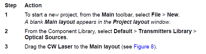

Figure 8: Adding a CW Laser to the Main layout
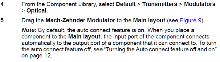
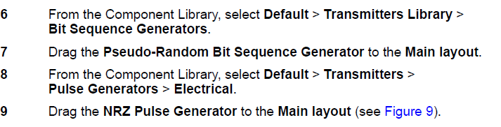

Figure 9: Adding components to the Main layout
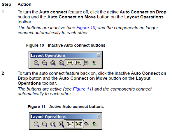
Auto connect feature
By default, the Auto Connect on Drop feature is active. There are two ways that components can auto connect:
- Auto Connect on Drop: When you place a component from the Component Library in the Main layout, the input port of the component connects automatically to the nearest output port of another component.
- Auto Connect on Move: When you move a component in the Main layout, the input port of the component connects automatically to the nearest output port of another component.
Turning the Auto connect feature off and on
To turn the Auto connect feature off and on, perform the following procedure.
Connecting components manually
The only connectable ports are those which have the same type of signal being transferred between them.
The exception to this rule is the ports that can be added to a sub-system and certain components in the library that have ports, which support any type of signal (for example, Forks).
Note: You can only connect output to input ports and vice versa.
![]()
Figure 12: Rubber Band Cursor
The rubber band cursor appears when you place the cursor over a port.
To connect components using the layout tool, perform the following procedure.
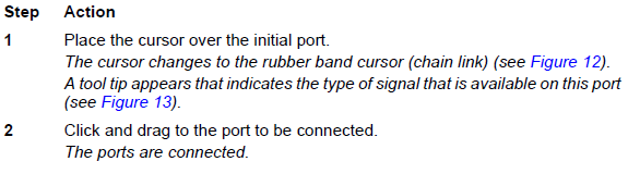

Figure 13: Connecting components symbol

Figure 14: Connecting ports
To connect the components, click on the port of one component and drag the connection to the port of a compatible component (see Figure 16).
a. Connect the Pseudo-Random Bit Sequence Generator output port to the NRZ Pulse Generator Bit Sequence input port.

Figure 15: Connecting components
b. Connect the NRZ Pulse Generator output port to the available Mach-Zehnder Modulator input port.
c. Connect the CW Laser output port to the Mach-Zehnder Modulator input port.

Figure 16: Connecting components
Visualizing the results
OptiSystem allows you to visualize simulation results in a number of ways. The Visualizer Library folder in the Component Library allows you to post process and display results from a simulation. The visualizer is categorized as an electrical or optical visualizer according to the input signal type.
For example, to visualize the electrical signal generated by the NRZ Pulse Generator in time domain, use an Oscilloscope Visualizer.
Visualizing the results
To visualize the results, perform the following procedures.
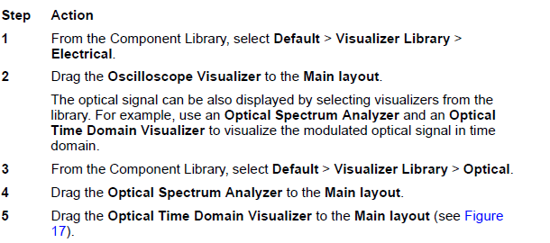

Figure 17: Visualizers in Main layout
Connecting visualizers
To visualize the signal from one component, you must connect the component output port to the visualizer input port.
You can connect more than one visualizer to one component output port. As a result, you can have multiple visualizers attached to the same component output port.
To connect visualizers, perform the following action.
Action
To connect the component and visualizers, click on the output port of the component and drag it to the input port of the visualizer (see Figure 18).
Note: You can only connect one component to a visualizer input port.
a. Connect the NRZ Pulse Generator output to the Oscilloscope Visualizer input port.
b. Connect the Mach-Zehnder Modulator output to the Optical Spectrum Analyzer input port and to the Optical Time Domain Visualizer input port.

Figure 18: Connecting components to visualizers
Visualizers and data monitors
When you connect a visualizer to a component output port, OptiSystem inserts a default data monitor to the component output port. You can then connect the component to the visualizer.
Note: Visualizers always connect to monitors. You can have multiple visualizers attached to the same component output port, because they are actually attached to the monitor, not to the component (see the Mach-Zehnder Modulator with connections to the OTDV and the OSD in Figure 19). Data monitors are represented by a rectangle around the component output port (see Figure 19 for examples of monitors on components).

Figure 19: Visualizers and monitors
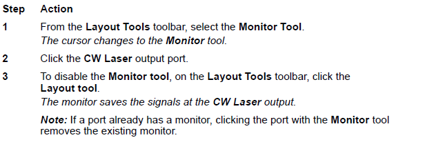
Connecting a monitor to a port
Visualizers post-process the data that the data monitor saves. You can connect a monitor to a port without connecting to a visualizer, and the monitor will save the data after the simulation ends. If you insert a monitor into a port before the simulation starts, you can connect visualizer to this monitor after the simulation ends without having to run the simulation again.
To connect a monitor to a port, perform the following procedure.
Component parameters
Viewing and editing component properties
To view the properties of a component, perform the following action.
Action
In the Main layout, double click the CW Laser.
The CW Laser Properties dialog box appears (see Figure 20).
Component parameters are organized by categories. The CW Laser has five parameter categories.
- Main — includes parameters for accessing a laser (Frequency, Power, Line width, Initial phase)
- Polarization
- Simulation
- Noise
- Random numbers

Figure 20: Component parameters
Each category has a set of parameters. Parameters have the following properties:
- Disp
- Name
- Value
- Units
- Mode
Display parameters in the layout
The first parameter property is Disp. When you select this property, the parameter name, value, and unit appear in the Main layout. For example, if you select Disp for Frequency and Power, these parameters appear in the Main layout (see Figure 21).

Figure 21: Displaying parameters in the Main layout
Parameter units
Some parameters, such as Frequency and Power, can have multiple units. Frequency can be in Hz, THz or nm, and Power can be in W, mW, or dBm (see Figure 22). The conversion is automatic.
Note: You must press Enter or click in another cell to update the values.

Figure 22: Parameter units
Changing parameter modes: arithmetic expressions
Each parameter can have three modes: Normal, Sweep and Script. Script mode allows you to enter arithmetic expressions and to access parameters that are defined globally.
To change parameter modes, perform the following procedure.
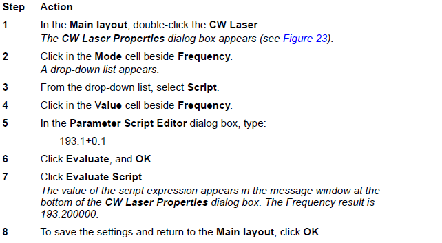

Figure 23: Scripted parameters
Accessing visualizer parameters
To access the parameters for a visualizer, perform the following procedure.
Note: You must right-click on a visualizer to access the parameters. Double-clicking on a visualizer brings up a dialog box to visualize the graphs and results generated during the simulation, not the parameters.
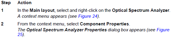

Figure 24: Layout menu

Figure 25: Visualizers parameter dialog
![]()
Running the simulation
OptiSystem allows you to control the calculation in three different ways:
- Calculate the whole project: all sweep iterations for multiple layouts
- Calculate all sweep iterations in the active layout: all sweep iterations for the current layout
- Calculate current sweep iteration: current sweep iteration for the current layout
By default, you will calculate the whole project, since there are currently no multiple layouts and no sweep iterations.
To run a simulation, perform the following procedure.
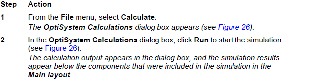

Figure 26: Running the simulation
Saving the simulation results
OptiSystem allows you to save the data from the monitors. This allows you to save the project file with the signals from the monitors. Next time you load the file, the visualizers will recalculate the graphs and results from the monitors.
To save the simulation results, perform the following procedure.
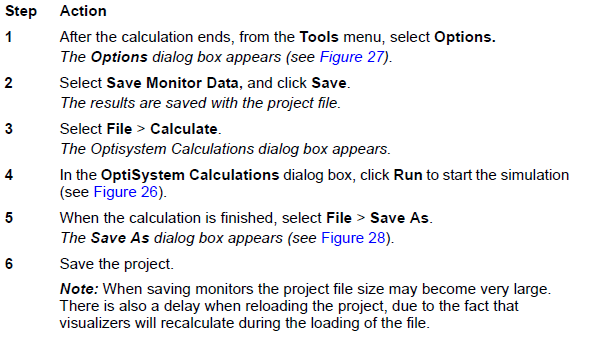

Figure 27: Options dialog box—Save Monitor Data selection

Figure 28: Save As dialog box
Displaying results from a visualizer
To display results from a visualizer, perform the following action.
Action
- Double-click a visualizer to view the graphs and results that the simulation generates.
Note: Double-click again to close the dialog box.
Oscilloscope
To visualize electrical signals in time domain with an oscilloscope (see Figure 29), perform the following action.
Action
Double-click the Oscilloscope Visualizer.
The Oscilloscope Visualizer dialog box appears.
Since OptiSystem can propagate the signal and noise separately, you can visualize the results separately. Use the tabs on the left side of the graph to select the representation that you want to view.
- Signal
- Noise
- Signal + Noise
- All

Figure 29: Oscilloscope
Optical Spectrum Analyzer
To visualize optical signals in frequency domain with an Optical Spectrum Analyzer (see Figure 30), perform the following action.
Action
- Double-click the Optical Spectrum Analyzer. The Optical Spectrum Analyzer dialog box appears.
Since OptiSystem uses a mixed signal representation, you can visualize the signal according to the representation. Use the tabs on the left side of the graph to select the representation that you want to view.
- Sampled
- Parameterized
- Noise
- All
To access the optical signal polarization, use the tabs at the bottom of the graph.
- Power: Total power
- Power X: Power from polarization X
- Power Y: Power from polarization Y

Figure 30: OSA
Optical Time Domain Visualizer
To visualize optical signals in time domain with an Optical Time Domain Visualizer (see Figure 31), perform the following procedure.
Action
- Double-click the Optical Time Domain Visualizer. The Optical Time Domain Visualizer dialog box appears.
In time domain, OptiSystem translates the optical signal and the power spectral density of the noise to numerical noise in time domain. Use the tabs at the bottom of the graph to select the representation that you want to view.
Power: Total power
Power X: Power from polarization X
Power Y: Power from polarization Y
Note: When you select polarization X or Y, you can also select to display the phase or chirp of the signal for that particular polarization.

Figure 31: Optical Time Domain Visualizer
Info-Window
When you open the Info-Window, it appears in the work area of a visualizer graph. By default, the Info-Window displays the current position (in database coordinates) of the cursor. When you zoom, pan, or trace the graph, the coordinates in the Info-Window change to reflect the coordinates of the cursor.
Accessing the Info-Window
To access the Info-Window, perform the following procedure.
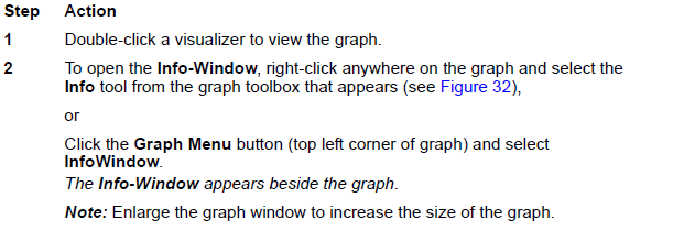

Figure 32: Graph toolbox
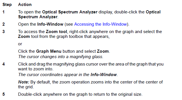
Zoom, Pan, and Trace tools
The Zoom, Pan, and Trace tools help you analyze and extract information from the graphs.
Zooming into a graph
To zoom into a graph, perform the following procedure.
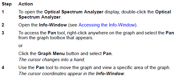
Panning a graph
To pan a graph and view a specific area, perform the following procedure.
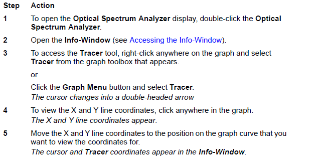
Tracing a graph
To trace a graph and obtain the values for each point in the graph, perform the following procedure.
Saving graphs
You can obtain the table of points with the values for each point in the graph and then save this as a test file. Copy the graph to the clipboard as a bitmap, or export the graph in different file formats — for example, metafile or bitmap.
To save a graph, perform the following procedure.
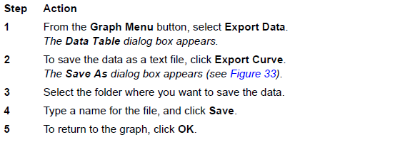

Figure 33: Graph menu dialog

Figure 34: Data Export dialog