
This lesson demonstrates the influence of stimulated Raman scattering on short soliton pulses.
The layout and its global parameters are shown in Figure 1.


Figure 1: Layout and global parameters

Figure 2: Setup for the Bit sequence generator

Figure 3: Setups for the Sech-pulse generator
The parameters of the nonlinear dispersive fiber component are shown in Figure 4.
The layout simulates N=2 soliton pulse propagation within five soliton periods [1].
The pulse width (FWHM) is 450.62fs, with the corresponding value of T0 being T0 ≈ (TFWHM/ 1.763) = 255.6fs.

Figure 4: Parameters of the nonlinear dispersive fiber component
 and spectrum (bottom)")
 and spectrum (bottom)")
Figure 5: Input pulse shape (top) and spectrum (bottom)
Figure 5 shows the input pulse shape and spectrum. The output (after five soliton periods of propagation) pulse shape and spectrum are shown in Figure 6. It can be seen that the effect of stimulated Raman scattering on the higher-order soliton is to split it into its constituents [1].
 pulse shape (top) and spectrum (bottom)")
 pulse shape (top) and spectrum (bottom)")
Figure 6: Output (at five soliton periods) pulse shape (top) and spectrum (bottom)
Moreover, the frequency domain manifestation of this effect (soliton self-frequency shift) can be clearly seen upon comparing the input and output pulse spectrum.
The normalized frequency shift:
![]()
agrees well with that presented in [1].
The same layout can be used to demonstrate the applicability of the approximation of the full Raman response of the material with the intrapulse Raman scattering in the case when the signal bandwidth is much narrower compared to the Raman gain spectrum [1], which is the case considered here. To achieve this we choose “Full Raman response” in the Nonlinear dispersive fiber (Non-linearities tab) (Figure 7).

Figure 7: Full Raman response in the nonlinear dispersive fiber
The rest of the setup remains unchanged. The obtained output spectrum is shown in Figure 8.

Figure 8: Output pulse spectrum at five soliton periods Full Raman response is used in the nonlinear dispersive fiber.
The remainder of this lesson demonstrates a phenomenon known as soliton self-frequency shift.
In order to do this, we make the following changes to the layout (see Figure 9):
 and output at 50 soliton periods (right) pulse spectra")
Figure 9: Input (left) and output at 50 soliton periods (right) pulse spectra
The normalized red shift of the soliton frequency is:
![]()
On the other hand, the same quantity if arrived at with the following expression [1]:
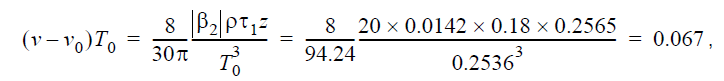
which agrees with the results we obtained.
Reference:
[1] G. P. Agrawal Nonlinear Fiber Optics, Academic Press (2001).