
This lesson demonstrates how OptiSystem can work with OptiGrating to design a proper dispersion compensation element in optical systems. The idea behind it is to use the additional possibilities provided by OptiGrating for design of fiber gratings.
The physical idea behind this compensation is following: creating of a linear chirped grating allows us to create a time delay between different spectral components of the signal.
For example, in SMF at 1.55 μm group velocity dispersion creates a negative chirp of the pulses, which means that the higher frequencies (which propagate faster) are in the leading part of the pulse and the lower (propagating slower) in the trailing one.
Because of this different velocity of propagation of different spectral components, the pulse spreads. If we create fiber grating with period linearly reducing along the grating, because of the fact that the higher frequencies will reflect after longer propagation in the grating, a time delay between lower and higher frequency components will appear which is just opposite to this created in the SMF.
Therefore propagating and reflecting our pulse in this device will allow to compensate the dispersion broadening of our pulse.
The dispersion coefficient Dg [ps/nm.km] for the linearly chirped fiber Bragg grating is given by the following simple expression [1]:
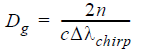
where n is the average mode index, c is light velocity, Δλchirp is the difference in the Bragg wavelengths at the two ends of the grating (note that this quantity is given by the total chirp parameter in the grating definition tab in the Grating Manager of OptiGrating).
In the first layout:
a. Linear chirped fiber Bragg grating. Linear chirped FBG.txt
The aim of the first layout is to accomplish dispersion compensation in OptiSystem with the help of a fiber grating with linear chirp generated in accordance with the above formula.
The project under consideration is in Figure 1.

Figure 1: Project Layout for dispersion compensation with fiber grating with linear chirp
For bit rate 40 Gb/s and with 0.5 times bit slot, in the Optical Gaussian pulse generator, an initial 12.5 ps pulse was generated and propagated in 10 km SMF. Initial pulse and output from the SMF pulses are shown in Figure 2 and Figure 3.

Figure 2: Initial pulse

Figure 3: Pulse after 10 km propagation in SMF
As a result of dispersion, the pulse width increases to approximately 50 ps. The accumulated dispersion after 10 km propagation in SMF is of 160 ps/nm.
In order to compensate for the accumulated dispersion, we will use FBG designed by means of the file Linear chirped FBG.ifo in OptiGrating. The corresponding data for the fiber and the grating is shown in Figure 4 and Figure 5.

Figure 4: Core data
Step-index fiber with the widths of the core (refractive index 1.46) and the cladding (refractive index 1.45) 2μm and 8μm, respectively.

Figure 5: Grating Definition dialog box
We consider linear chirped FBG with chirped bandwidth Δλchirp = 0.35nm . If we assume the average mode index ~ 1.46 in accordance with the above formula, we get the required length of the grating from ~ 6 mm for the compensation of 160 ps/nm accumulated dispersion in the SMF.
In the presented calculation, we have used the grating with slightly larger length ~ 1.6 cm. Obtained results are saved in the file Linear chirped FBG.txt. This file is loaded in the Linear Chirped FBG component.
The obtained result of compensation is shown in Figure 6.

Figure 6: Pulse after dispersion compensation with linear chirped FBG
As we see, with designed by means of FBG practically complete dispersion compensation was achieved.
b. Fiber Bragg grating designed by means of inverse scattering algorithm
The aim of this layout is to perform dispersion compensation with the help of a fiber Bragg grating, designed with the inverse scattering algorithm of OptiGrating.
Such FBG is created with the help of OptiGrating’s file Lesson7.oad. The requirement in designing of this FBG is that it has to produce accumulated dispersion of -160 ps/nm. The obtained spectrum is saved in Complex Spectrum 7 Lesson.txt.

Figure 7: Project Layout for dispersion compensation with FBG with inverse scattering algorithm
The result from the dispersion compensation of accumulated dispersion in SMF is shown in Figure 8.

Figure 8: Pulse after dispersion compensation with fiber grating FBG generated in OptiGrating with inverse scattering algorithm and – 160 ps/nm accumulated dispersion
As we see, designed in this way, FBG allows to reduce the pulse width to approximately 17 ps.
To sum up, in this lesson we have demonstrated how the dispersion compensation in OptiSystem can be achieved using a reflection spectrum obtained with the gratings designed by means of OptiGrating.
References:
[1] G.P. Agrawal, “Fiber-optics communication systems”, Wiley Inter-Science, 2002