
In the first lesson, you will learn how to design a Fiber Bragg Grating with chirp and
apodization. Such a grating finds application in fiber dispersion compensation.
| S.1 | |
| The first thing you will do is to open a new project. Then, you will choose one of the five available modules to work with: Single Fiber, Fiber Coupler, Single Waveguide, Waveguide Coupler, and Other Waveguide. |
To select the Single Fiber Module
| 1 | File > New. |
| 2 | In the New dialog box, click the Single Fiber option.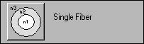 Note: You can also open a new project by clicking the New button on the Toolbar. Note: You can also open a new project by clicking the New button on the Toolbar. |
| S.2 | |
| Next, you will define certain parameters for the Single Fiber. You will do that in the Single Fiber dialog box in which you can set the following characteristics: Index Profile, Photosensitivity Profile, Number Of Points In Mesh, Central Wavelength, etc. |
To open the Single Fiber dialog box
| 1 | In the Project Window, click the Fiber/Waveguide Parameters button. |
The Single Fiber dialog box appears on the screen.
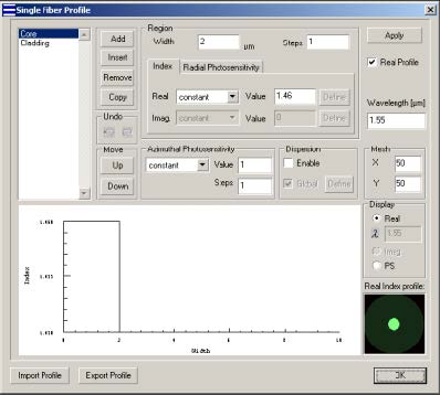
Note: Since you are going to use the default parameters, you don’t have to
change any of the predefined options.
| 2 | Click OK to close the Single Fiber dialog box. |
| S.3 | |
| In this step, you will access a list of the calculated modes of your Fiber/Waveguide structure. The fiber you use is a single mode fiber.To see a list of the calculated modes | |
| 1 | From the Parameters Menu, click Mode. |
| 2 | Make sure that the Input Amplitude is set to 1 and the Phase is set to 0. |
| 3 | Click the OK button. |
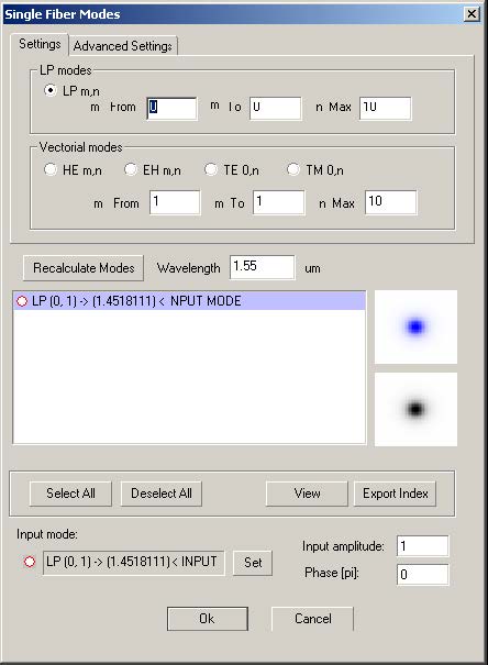
Note: If you have chosen to work with the Single Fiber module or the Single
Waveguide module, you will see that there is only one list of modes in the Modes
dialog box. If you are working with other modules, you will see that there are two
lists available in the dialog box.
| S.4 | |
| In this step, you will learn how to open the Grating Manager dialog box and how to access the Grating Definition dialog box in which you can define the parameters of each grating. The Grating Manager gives you a list of your grating objects (and some important information about those objects) and allows you to add, remove, or copy gratings or phase shifts. |
To open the Grating manager dialog box
| 1 | From the Parameters Menu, click on the Grating… |
| 2 | In the Grating Manager dialog box, double-click the Grating 1 object to open the Grating Definition dialog box.Note: To open the Grating Definition dialog box, you can also click the Edit Item button. |
| S.5 | |
| In this step, you will define the parameters of the grating you’re working with in the Grating Definition dialog box. |
To define the grating’s parameters
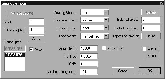
| 1 | In the Grating Definition dialog box, from the Grating Shape list box, choose Sine. |
| 2 | From the Average Index dialog box, choose Uniform. |
| 3 | In the Index Change box, make sure the index is set to 0. |
| 4 | From the Period Chirp list box, choose Linear. |
| 5 | In the Total Chirp box, type 2. |
| 6 | From the Apodization list box, choose User Defined. |
| 7 | In the Ind. Mod. box, type 0.0006. |
| 8 | In the Number of Segments box, type 101.Note: You will notice that for some of the parameters you can use either the predefined functions or the User Defined options. Notice that when you choose the User Defined option form the Apodization list box, the Define button is enabled.
|
| S.6 | |
| In this step, you will learn how to program functions in the User Defined dialog box. The User Defined dialog box allows you to program functions by using Basic syntax and to test visually the function by pressing the Display button. At the end of this step, you will have defined all the necessary parameters for the Fiber Bragg grating. |
To program and test functions
| 1 | In the Grating Definition dialog box, click the enabled Define button (next to the Taper’s Parameters option). |
| 2 | In the User Defined Function dialog box, delete everything from the Edit window (where you have a function already defined by default) and write the following function: w = 0.7 |
exp(-(2*(x-Length/2)/(Length*w))^4)
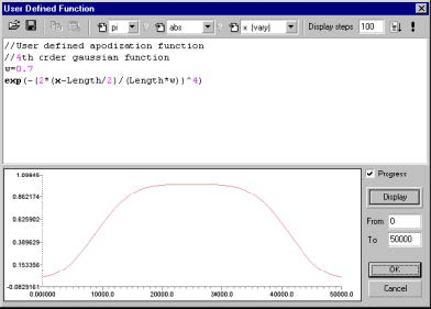
| 3 | Click the Display button to see a new curve with the parameters you have defined in the Grating Definition dialog box. |
Note: When you change the value of “w” and click the Display button, you will see a different curve. You may want to experiment with different values before closing the User Defined Function dialog box.
- Anything written on a line after the // command is ignored.
4Click the OK button to close the User Defined Function dialog box.5In the Grating Definition dialog box, click the OK button.6In the Grating Manager dialog box, click the OK button to return to the Project Window.
| S.7 | |
| Having defined all the necessary parameters for the Fiber Bragg grating, you will now learn how work in the Multiple View window.In the Project Window, you have access to different Parameter buttons, displayed on the left side of the Project Window. You can choose from several Calculation options, listed in the Calculation list box; you can use the color button, placed on the small Toolbar; and you can use the Display tabs, placed at the bottom of the Graph window. |
To see the calculation results
| 1 | From the Calculation list box, choose Propagation. |
| 2 | In the Propag. step edit box, type 500 |
| 3 | Click the Calculate button to see the results. |
To use the color buttons
| 1 | Click anywhere in the Graph window. |
| 2 | On the small toolbar, press the Red button to see the Transmitted Power curve. |
| 3 | Press the Blue button to see the Reflected Power curve.Note: Each color represents a different curve. In the example above, only two color buttons can be enabled because there are only two curves available.
|
| S.8 | |
| There are several Display tabs available in the Multiple View window. Each tab represents a different graph. Depending on the Module you are using and the options you have chosen, some of the tabs may be disabled. For example, the 3D Display tab is enabled only when you are performing a Propagation calculation. |
To use the Display tabs
| 1 | In the Project Window, click in the Graph window. |
| 2 | Click the 3D Display tab. |
| 3 | In the Graph window, click the right mouse button to see the pop-up menu.Note: The pop-up menu allows you to use several commands: Crossection Monitor (to see across sections), Display Properties, and Print Graph.  |
| S.9 | |
| In this step, you will learn how to use the different calculation options and how to do simple calculations. For this purpose, you will use the calculation options in the Calculation list box that contains the most often used calculation options. |
To Calculate spectral characteristics
| 1 | In the Multiple View window, click the Power tab. |
| 2 | From the Calculation list box, choose Spectrum. |
| 3 | Select wavelength range from 1.545um to 1.555um, and set the Steps to 500. |
| 4 | Press the Calculate button to calculate the spectral characteristics. |
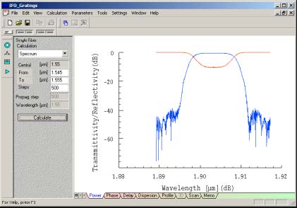
| 5 | Right click on the graph. |
| 6 | From the list, choose Axis Properties. |
| 7 | Select the Left Y axis tab, then deselect the Show as dB box. |
| 8 | Click OK. The graph will change automatically.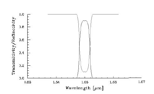 Note: Notice that the parameters in the Calculation section change according to the option you have chosen from the Calculation list box. Note: Notice that the parameters in the Calculation section change according to the option you have chosen from the Calculation list box. |
| S.10 | |
| OptiGrating allows you to measure automatically full width at half maximum. To do so, in this step you will use the FWHM tool. |
To use the FWHM tool
| 1 | Click once on the display window. Select the Reflection curve by clicking the red button on the tool bar. |
| 2 | Right click on the graph. |
| 3 | From the list, choose Axis Properties. |
| 4 | Select the Left Y axis tab, then deselect the Show as dB box. |
| 5 | Click OK. |
| 6 | Select FWHM from the Tools drop down menu to display the ‘Tools’ dialog box. |
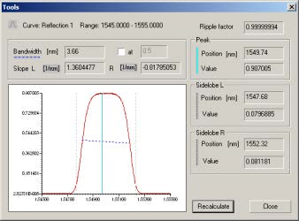
| 7 | In the Tools dialog box, to calculate the bandwidth at half of the maximum, select the At check box beside bandwidth. |
| 8 | Enter 0.5 in the box next to the At check box. |
| 9 | Click Recalculate |
| 10 | Click the Close button to close the dialog box.Note: In the Tools dialog box, you can calculate not only the bandwidth at half of the maximum: if you enable the At check box, you can enter any desired y-axis absolute position in the box and click the Recalculate button.
|
| S.11 | |
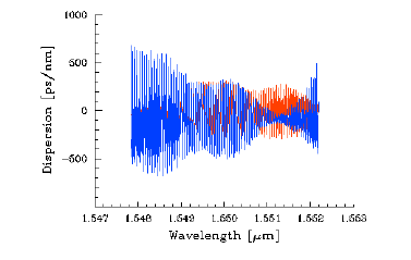
| In this step, you will see the Cumulative Phase graph, the Delay graph, and the Dispersion graph. |
To see the Cumulative Phase graph
| 1 | In the Project Window, type 1.54784 in the From box. |
| 2 | In the To box, type 1.5522. |
| 3 | In the Steps box, type 800.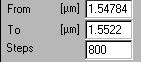 |
| 4 | Make sure both the Reflection and Transmission buttons are selected. |
| 5 | Click the Calculate button. |
| 6 | In the graph window, click the Phase tab. |
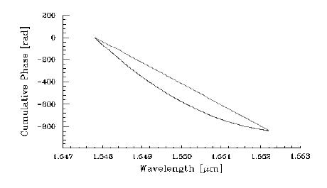
Note: By default, the Phase is cumulative. To toggle between the Cumulative
Phase and standard phase, double click the left mouse button and from the popup
menu, click Cumulative Phase.
To see the Delay graph
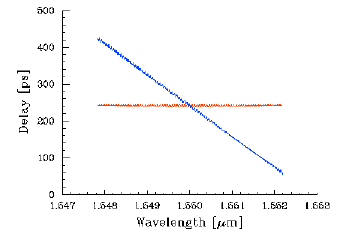
In the Multiple view window, click the Delay tab.
To see the Dispersion graph
In the Multiple view window, click the Dispersion tab.
| S.12 | |
| In this step, you will choose the Pulse Response Calculation option, define some of the Pulse Response characteristics, and do a simple calculation. |
To define Pulse Response characteristics
| 1 | Click in the graph window. |
| 2 | From the Calculation list box, choose Pulse Response. You will notice that the Define button is enabled. |
| 3 | In the Steps box, type 511. |
| 4 | In the Time Span box, type 200. |
| 5 | In the Wavelength box, type 1.55. |
| 6 | Click the Define button. |
| 7 | In the Pulse Response dialog box, from the Input Pulse list box, choose Gaussian. |
| 8 | In the Intensity FWHM box, type 10 and click the OK button. |
| 9 | In the Project Window, click the Calculate button.Note: You do not need to enable the Link check box at this point. |
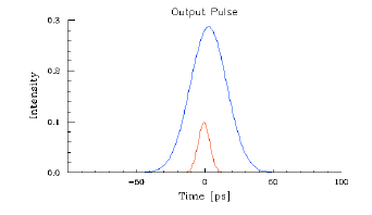
| S.13 | |
| In this step, you will explore some of the graphs for Pulse Response. You can see Input Pulse, Input Spectrum, Grating Spectrum, and Output Pulse. |
To view the Output graph
In the Multiple view window, click the Output tab.
To see the Profile graph
In the Multiple view window, click the Profile tab.
To see the Profile graph
In the Multiple view window, click the Profile tab.
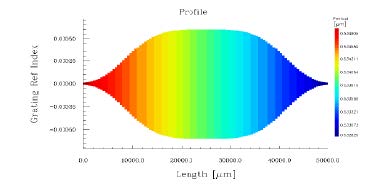
- The Profile tab displays your grating characteristics defined in the Grating Manager and the Grating Definitions dialog boxes. You can display all characteristics separately, as a 2D graph, or combined, as a Profile graph.
- To switch between characteristics, click the right mouse button and from the popup menu choose the desired option.
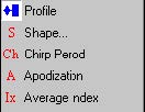
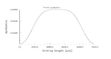
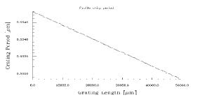
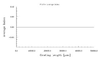
What do you see on the Profile graph?
Select Apodization
On the y-axis of the Profile graph, you see the grating Refractive Index that is
determined by Apodization:
Select Profile Chirp Period
On the y-axis of the Profile graph, you see the grating period that is determined by the
Grating Period Chirp:
Select Average Index
The profile is also determined by the Average Index. Since you have selected Uniform
Average Index, the Profile is positioned to 1.46 as Core Refractive Index:
This ends Lesson 1. You may now proceed to Lesson 2 that uses the grating profile
from Lesson 1. Otherwise, save your work in order to be able to do the next tutorial
lesson later. To save your work, select Save As from the File menu and enter a file
name (for example, Lesson1.ifo).