
Next Generation 3D-FDTD Solver
OptiOmega 3D-FDTD solver implements the Finite-Difference Time-Domain (FDTD) algorithm in second-order central difference in both time and space to solve Maxwell’s equations, specifically optimized for the simulation of integrated photonic devices. It uses the Perfectly Matched Layer (CPML) boundary conditions for accurate open region simulations. The implementation is grounded in the foundational works by Taflove [1], Hagness [1], Elsherbeni[2], and Demir[2], and adapts their rigorous mathematical formulation to a highly automated and scalable simulation environment. It’s a super fast simulator which uses the Graphics Processing Unit (GPU) to compute the performance of photonic structures. In addition, OptiOmega is able to take advantage of running on cloud services like AWS and Azure allowing affordable access to very fast GPU’s with high RAM.
With the upcoming challenges of complexity in the integrated systems, the accurate design and analysis of the photonic devices, within a short time frame, is a must for any organization to thrive in the ever-leading photonics domain. OptiOmega offers a complete vectorial solution at a turbo speed (> 100x faster than a normal CPU), thereby, drastically reducing the computational time of the simulations. It is a complete python language based simulator, with a wide range of automated features which minimizes manual labor during simulation setup. It generates the optical S-parameters and stores the results in .HDF5 format which can be used for post-processing by taking leverage of python libraries. It also offers the optimization of the photonic devices by making use of Particle Swarm Optimization (PSO) algorithm.
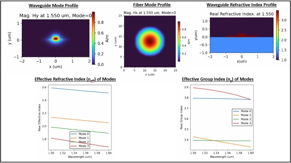
OptiOmega comes bundled with the VFD mode solver which implements a full-vector finite-difference mode-solving algorithm for analyzing dielectric waveguides, based on the method presented by Fallahkhair et al [3]. It is designed to compute the guided modes of anisotropic, lossy, and inhomogeneous dielectric structures in two dimensions (2D), making it ideal for modeling complex photonic components. It runs on the CPU and allows researchers and engineers to analyze the modes, field profiles, effective refractive indices (neff) and group indices (ng) of the waveguide based structures and complex shapes. This tool is important and leads as a foundation towards the development of robust photonic complex structures.
The interoperability of OptiOmega with other powerful chip and system level simulator tools like OptiSPICE and OptiSystem, within Optiwave suite, allows users to characterize and validate the figure of merits of the simulated photonic devices in the real world application scenario. Users can import the computed S-parameters and modal data into these tools and build and analyze the performance of their chip/system level circuit, by running frequency or time domain simulations, with the aid of vast opto-electronic and visualizer’s library.
Few standout features of OptiOmega are as follows: –
- The entire workflow of OptiOmega is based on the python language, which allows users to automate the simulation process and take leverage of several python libraries for data analysis.
- OptiOmega runs on the standalone GPU and also on the cloud services which makes the computational time 100x faster than a similarly priced CPU.
- It allows GDSII and STL mask layout imports of the photonic devices.
- It has automatic port detection and enumeration feature, without the need of ports specification.
- The time window setting has the auto-shutoff feature.
OptiOmega Overview
OptiOmega is a collection of products specialized for photonic integrated circuit simulation. It automates the design flow for generating compact models from device level simulations. The software package includes two solvers that can be used via python scripting: Vector Finite Difference (VFD) Mode Solver and Finite Difference Time Domain (FDTD) Electromagnetic Solver.
The FDTD electromagnetic solver implements the Finite-Difference Time-Domain algorithm for solving Maxwell’s equations in time and space, specifically optimized for the simulation of integrated photonic devices. It supports linear, isotropic, non-dispersive materials and provides advanced features tailored to photonic circuit design, such as automatic mode injection, port detection, and S-parameter extraction. It is a GPU accelerated simulator which aids in achieving ultra-fast computational speeds which can either run locally or run on the cloud services like AWS and Azure allowing affordable access to very fast GPU’s with high RAM.
Whereas, the VFD Mode solver implements a full-vector finite-difference mode-solving algorithm for designing and analyzing dielectric waveguides and complex shapes. Unlike scalar or semi-vectorial approximations, this solver fully resolves the vectorial coupling of the electromagnetic field, supporting anisotropic dielectric permittivity and complex materials with loss. It computes the guided modes of anisotropic, lossy, and inhomogeneous dielectric structures in two dimensions (2D).
APPLICATIONS
The VFD solver aids in designing of:
- Silicon photonics and integrated optical waveguides
- Photonic crystal fibers and birefringent fibers
- Structures comprising of electro-optic & magneto-optic materials and materials with loss/gain.
- Nano-photonic waveguides
- High index contrast devices by analysis of hybrid modes.
The 3D-FDTD solver aids in designing of:
- Silicon photonics and integrated optical circuits
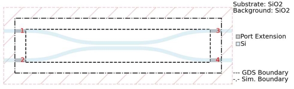
- Passive photonic devices such as couplers, splitters, multiplexers and filters.
- Devices such as waveguide tapering, crossings, resonators, MMIs, junctions, etc.
KEY Features
VFD mode solver
- It solves for full-vector field i.e. for all components (Ex, Ey, Ez) of the electric field.
- Handles diagonal tensor (anisotropic) permittivity (εx, εy, εz).
- It supports lossy materials and leaky modes.
- Uses central-difference schemes on structured Cartesian grids.
- Perfect Electric Conductor (PEC) boundary condition.
- Allows GDSII mask import generated by any mask layout tool.
- Allows material import from Sellmeier model, constant refractive index values, material data from info and experimental data.
- Handles sidewall angles and user defined sidewall functions.
- It solves for mode profiles and calculates effective indices and group indices.
- Accurately identifies all types of guided modes such as TE, TM, and hybrid modes.
3D-FDTD Solver:
- Time-domain Maxwell solver using second-order central difference in both time and space.
- Convolutional Perfectly Matched Layer (CPML) boundary conditions for accurate open-region simulations. It is used to prevent artificial reflections at simulation domain boundaries.
- Reads standard GDSII and STL layout files to define device geometry.
- Automatic port detection and classification.
- Mode solver integration for accurate injection and extraction. It injects single mode using computed eigenmodes.
- Handles automatically adjusted parametric sweeps.
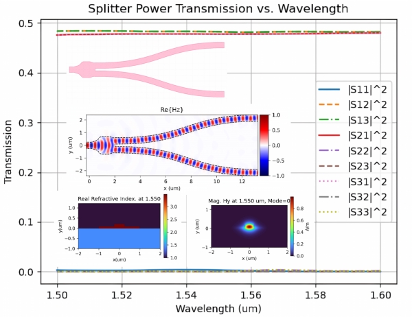
- Computes scattering parameters (S-matrix) from time-domain data for each iteration and automatically exports results in standard .SNP format.
- All simulations data, field snapshots and metadata are stored in .HDF5 format for efficient post-processing.
- OptiOmega allows defining constant refractive index material values as well as from Sellmeier model. It’s in-built function also allows to import material data directly from info and a foundry based experimental data.
- Handles sidewall angles and user defined sidewall functions.
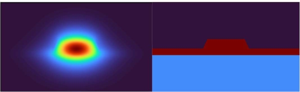
- It has sub-pixel averaging feature that allows better description of the material distribution, by reducing the stair-casing of the permittivity profile and minimizing unwanted reflections. Sub-pixel averaging when turned ON, allows to achieve precise and accurate results even with coarse mesh settings, thereby reducing computational time.
![]()
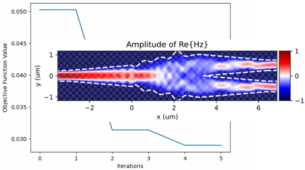
- Supports device optimization based on the Particle Swarm Optimization (PSO) algorithm, with the aid of various python based optimization packages.
- Automatically sets the simulation domain size based on the geometry.
- The position placement, size and settings of the input plane source and the mode monitors are all automated.
- The simulation time window setting has an auto-shutoff feature which automatically computes the simulation when the fields propagating inside are well converged.
- The feature of reciprocal ports detection helps in computing the S-parameters of the devices having reciprocal ports by injecting mode from only 1 port instead of injecting mode from all the ports. This aids in reducing computational time.
- OptiOmega’s automated features with minimal human intervention allows simulating multiple complex integrated photonic structures at once, with high accuracy and with very low computational time.
Software Interoperability
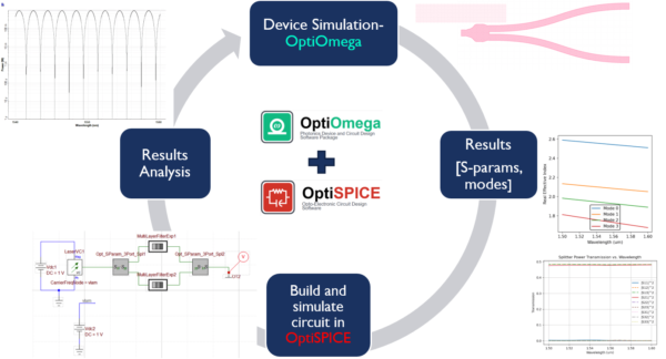
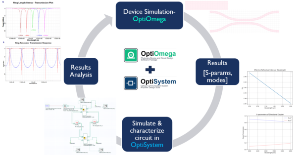
OptiOmega allows the software interworking internally with other Optiwave simulation tools such as: OptiSPICE and OptiSystem. OptiSPICE is a SPICE engine based electro-optic circuit simulator that allows to simulate chip level circuits in both frequency and time-domain. OptiSystem aids in building and characterizing the device/PIC performance at a system level. The photonic devices are simulated using OptiOmega and the generated results in the form of S-parameters (touchstone format) and modal data (neff and ng) are used to build the PICs or system level circuits inside OptiSPICE/OptiSystem. The frequency or time domain simulations are carried out for the circuits that helps in validating the device performance.
[1] Susan C. Hagness, Allen Taflove, “Computational Electrodynamics: The Finite-Difference Time-Domain Method”, 3rd Edition, Artech House, 2005. ISBN: 9781580538329
[2] A. Z. Elsherbeni, V. Demir, “The Finite-Difference Time-Domain Method for Electromagnetics with MATLAB® Simulations”, 2nd Edition, SciTech Publishing, 2015. ISBN: 9781613531754
[3] A. B. Fallahkhair, K. S. Li, and T. E. Murphy, “Vector Finite Difference Modesolver for Anisotropic Dielectric Waveguides”, Journal of Lightwave Technology, Vol. 26, No. 11, pp. 1423–1431, 2008.