
In a waveguide, light propagates in the form of modes. OptiGrating 4.2 uses LP Fiber modes, Vector Fiber modes, and Slab Waveguide modes.
LP Fiber Modes
The designation of Linearly Polarized (LP) Fiber modes is based on the assumption of weak guidance. Weakly guiding fibers have a small difference between core and cladding refractive index.
The LP (m, n) modes are designated by two numbers:
1 m – azimuthal number
2 n – orbital number
where m=0, 1, 2, … and n=1, 2, ….
Both guided and cladding modes of arbitrary circular symmetric refractive index profiles are calculated either by the accurate finite difference method or by the analytical method (step index profile). The fundamental mode of fiber is LP (0,1).
Vector Fiber Modes
The designation of Vector Fiber modes TE, TM, EH, and HE follows the convention:
1 TE(0,n) – transverse electric family of modes
2 TM(0,n) – transverse magnetic family of modes
3 EH(m, n) – hybrid family of modes
4 HE(m, n) – hybrid family of modes
where m>0 and n=1, 2, … .
In OptiGrating 4.2, the vector modes are calculated only for the step-index fiber. The step index calculations are based on the analytical approach. The fundamental mode of the stepindex fiber is HE (1,1).
Slab Waveguide Modes
The Slab Waveguide modes are the following:
1 TE(m) – transverse electric family of modes, m=0, 1, 2, …
2 TM(m) – transverse magnetic family of modes, m=0, 1, 2, …
The modes of a slab waveguide with arbitrary refractive index profile are calculated
either by the Transfer Matrix Method or by the analytical method (step index profile).
The fundamental mode is TE (0) or TM (0).
Mode Solver
Near the end of any calculation that finds the modes of an optical waveguide, it is
necessary to find the solution of an equation. This equation is a function of the propagation constant β and typically includes mixed trigonometric and exponential functions. Therefore a numerical solution, rather than an analytic one, is sought. For waveguides composed of lossless materials, the proper modes are easy to find since they are real numbers. Simple numerical routines need only to be provided with an interval on the real axis where the solutions can be expected, and it is a simple matter to find them all. On the other hand, in the case of leaky waveguides, or in the case of waveguides composed of lossy materials, the equation may still have solutions, but with β in the complex plane. These solutions are not proper modes, in the sense that the corresponding solutions for the electromagnetic fields are orthogonal to each other, or even (in the case of leaky modes) localised. Nevertheless, the electromagnetic field associated with this complex solution is still a valid solution of
Maxwell’s equations, and is relevant because it is often a good approximation to the
field seen for this waveguide in practice.
The numerical procedure for the so-called complex modes is more difficult, as the
search space is two dimensional. However, OptiGrating Version 4.2 uses an
advanced technique for finding these solutions. The user must specify a region in the
complex plane by giving limits to the imaginary values as well as the real ones. This
defines a rectangular shaped contour in the complex β plane. By one of the theorems
of Cauchy, the number of zeros of a function (minus the number of poles) enclosed in
a closed contour in a complex plane is given by the contour integral
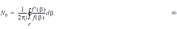
OptiGrating performs the contour integral numerically, and uses the above formula to
determine the number of complex modes to be found within the given limits. The
calculation of the modes is aided by the numerical evaluation of the following integrals
at the same time
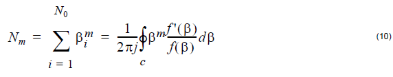
for m = 1, 2, 3, … N0. In fact, knowledge of the Nm allows the construction of a
polynomial that has the same roots as ƒ(β). The roots of the polynomial are then
solved by standard techniques such as Laguerre’s method. A detailed description of
the method can be found in the Reference [1].