
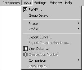
The Tools menu gives you quick and easy access to the following OptiGrating tools:
FWHM Tools
Automatically calculates the Full Width At Half Maximum (FWHM) of the current.
Group Delay
Automatically calculates the group delay slope, GDD, and ripple.
Phase
Selects the Phase Display mode when you are working with Phase graphs. You can
toggle between the Circular Phase display and the Cumulative Phase display.
Profile
Selects the mode of the Grating Profile display when you are working with Profile
graphs. You can toggle between the display of Shape, Chirp, and Apodization.
Export Curve
Exports a graph curve into one of the following two formats: Text or BPM_CAD View
2D.
Export Complex Spectrum
Exports complex spectrum data into one of the following three formats: Text,
BPM_CAD view 2D, or Optisys.
View Data
Displays the Data table.
Crossection Monitor
Displays a 2D cut from a 3D Propagation graph.
Comparison
‘Curve load…’: Reads data from a file and plots the data on the current view
‘Curve clear’: Clears the curve created by the ‘Curve Load’ option.
Note: You can also get access to some of the Tools menu by double clicking a
graph with the left mouse button.
FWHM
File: New > Module option > Tools: FWHM
Using the FWHM Command
The FWHM command helps you calculate the Full Width At Half Maximum (FWHM)
characteristics.
To perform a Full Width At Half Maximum calculation
| 1 | Click the graph you are currently working with. |
| 2 | From the Tools menu, click FWHM. |
| 3 | In the Tools dialog box, enter the desired values, click the Recalculate button, and then click the OK button. |
Note: The curve to be recalculated is the first visible curve in the graphic window.
If you would like to measure another curve, you have to disable the rest of the
curves by using the color buttons on the Toolbar.
![]()
The FWHM Tools dialog box
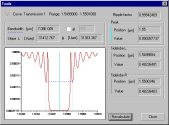
FWHM Tools enables you to measure the width, slope, ripple factor, and sidelobes of
a curve. The tools are most useful to characterize curves in the spectral domain;
however, they can also be used to measure curves in the time domain.
Note: The definitions below refer to a typical reflection curve with a central peak
surrounded by sidelobes and ripples. In characterizing a typical transmission
curve with a pronounced main minimum instead of a main peak, one should reinterpret
the definitions accordingly: maximum becomes minimum, etc.
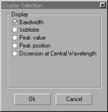
Bandwidth
By default, when the At option is not selected, the bandwidth is defined as the full
width at half maximum (FWHM). In the selected graph region, the vertical offset from
the bottom is excluded from this default measurement. If the At option is selected, the
bandwidth is defined as the full width at the given height.
Slope
The slope is defined as the first derivative of the curve at a given position. There are
two default horizontal positions for the slope measurement. They are determined by
the cross-section of the curve and the horizontal line used to measure the bandwidth.
Slope L is the slope at the left cross-point.
Slope R is the slope at the right cross-point.
Peak
Peak Position is the horizontal position of the maximum value.
Peak Value is the maximum value of the curve.
Ripple Factor
Ripple Factor is defined by:

where Ymax is the maximum value of the curve, Ymin is the minimum value of the
curve in the selected region. The best way to determine the ripple factor is to limit the
selected region to the ripple section only, that is, excluding the main peak.
Sidelobe
Sidelobe is defined as the maximum peak outside the main peak.
Sidelobe L is the left sidelobe
Sidelobe R is the right sidelobe
Sidelobe Position is the horizontal position of the sidelobe maximum
Sidelobe Value is the value of the sidelobe maximum
Group Delay
The Group Delay tool is used for grating dispersion management.
To open the Group Delay Tool
| 1 | File > New. |
| 2 | Select one of the options. |
| 3 | Click the Calculate button on the left. |
| 4 | Choose Spectrum from the drop-down menu. |
| 5 | To activate Group Delay, either the Phase, Delay, Dispersion, or Scan tabs must be selected. |
| 6 | Once a tab is selected, Tools > Group Delay, or select the Group Delay icon on the task bar beside the FWHM Tool icon. |
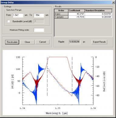
Spectrum Range
Set the wavelength delay range in the From and To boxes. This allows for more
freedom when determining where the delay begins and where it ends as indicated by
the vertical black lines. Click Recalculate to see changes
Bandwidth Level
To activate, select box to left of Bandwidth Level. This offers a close approximation of
the beginning and end points of the delay. You may enter different bandwidth levels
in right-hand box to further refine selection. Click Recalculate to see changes.
Maximum Fitting order
To get the most accurate results from the Group Delay tool, use Maximum Fitting
Order to trace the delay itself. By changing this number, you are better able to map
its length. Each step is listed in the Results box, showing both the Coefficients and
the Standard Deviations of the delay. Click Recalculate to see results.
Export Curve
File: New > Module option > Tools: Export Curve
Using the Export Curve Command
The Export Curve command allows you to export a graph curve into a text format or
a BPM, CAD View 2D format.
To define the Export Curve options
| 1 | Click the graph you are currently working with. |
| 2 | From the Tools menu, click Export Curve to open the export Curve dialog box. |
| 3 | In the Export Curve dialog box, choose the graph component you want to export: Transmission 1, Transmission 2, Reflection 1, or Reflection 2. |
| 4 | From the Export Format list box, choose either Text or BPM_CAD View 2D. |
| 5 | Click the Export button. Note: The Text format is x y. 0.000000e+000 1.000000e+000 8.313872e+001 9.999998e-001 1.662774e+002 9.999993e-001 2.494162e+002 9.999984e-001 …..The BPM_CAD native format (*.dat) is almost the same as the Text format, but it contains additional information, such as the number of points (in the example below, there are 501 points) in header: BCF2DPC 501 0.000000e+000 1.000000e+000 8.313872e+001 9.999998e-001 1.662774e+002 9.999993e-001 2.494162e+002 9.999984e-001 |
Crossection Monitor
File: New > Module option > Tools: Crossection Monitor
Using the Crossection Monitor command
| 1 | Click the graph you are currently working with. |
| 2 | From the Calculation list box, choose Propagation. |
| 3 | In the graph window, click the 3D tab. |
| 4 | From the Tools menu, click Crossection Monitor to open the Crossection Monitor dialog box. |
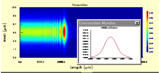
| 5 | Click the 3D graph with the left mouse button and holding down the button drag the mouse in x direction until you see a cutting line and a cross section appearing in the graph window. |
Note: You can resize the Crossection Monitor dialog box to suit your preferences.
If you click the right mouse button at the cross section of the coordinates displayed in
the Crossection Monitor dialog box, a pop-up menu opens which allows you to use
the Normalize To Maximum command or the Print command.
The Normalize To Maximum command will maximize the Crossection Monitor dialog
box, and you will be able to see the graph in detail.