
File: New > Single Fiber
The Single Fiber Module
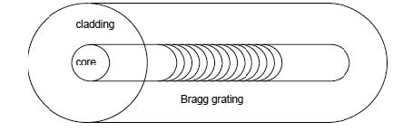
You use the Single Fiber module to model a fiber with arbitrary radial symmetry while
the grating can be placed anywhere in the fiber. OptiGrating allows you to adjust both
the fiber dimensions and refractive index profile and photosensitivity profile.
You can simulate the grating assisted coupling between forward and backward
propagating modes. There are two mode options available: LP modes or full, vector
modes (HE, EH, TE, or TM) of the fiber. The vector mode option is only available for
step-index fiber. The Single Fiber module finds application in WDM selective and
add/drop filters, dispersion compensators, long period fiber grating filters for EDFA
gain flattening, and sensors.
To choose the Single Fiber module
| 1 | File > New. |
| 2 | In the New dialog box, click Single Fiber. |
The Single Fiber Profile Dialog Box
In this dialog box, you enter the main data concerning the fiber dimensions: index
profile and photosensitivity profile.
To open the Single Fiber dialog box
| 1 | In the Project window, click the Fiber/Waveguide Parameters button. |
The Single Fiber Profile dialog box options are described below.
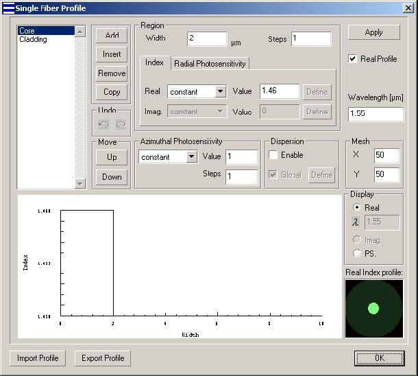
List of Regions
Shows the index radial regions by their names.
Add
Adds a region to the bottom of the list.
Insert
Adds a region immediately under the highlighted point on the list
Remove
Deletes the selected region from the list
Undo
Left undo arrow deletes previous steps. Right redo arrow replaces deleted steps.
Up
Moves the selected region one position up the list.
Down
Moves the selected region one position down the list.
Width
Enter the width of the selected region in microns.
Steps
Enter the number of steps for discretization of the index profile function.
Index tab
Real
Select one of the following options for the real index profile within the current region:
Constant – Constant value of the real refractive index
Linear
Parabolic
Gaussian
Exponential
Alpha-peak
Alpha-dip
User Function – Functional dependence of the index, where the function is defined or programmed using the powerful Script Language environment.
The notation convention for these functions is described in the Technical Background,
section Index Profile of Fibers. Conventionally, the functions’ argument is the radial
local distance that is zero at the beginning of the region and is equal to the Width
value at the end of the region.
Value (for Real Index)
Numerical data entry box – Present when the constant real index option is selected.
Enter the real refractive index value for the selected region.
Define (for Real Index)
Present when the Function or User Function option is selected. Press the Define
button to specify the function. For the built-in functions, a dialog box related to one of
the predefined functions appears. For the User Function option, pressing the Define
button launches the User Defined Function script programming environment.
Imag.
This option is available when the Real Profile check box is unchecked.
Select one of the following options for the imaginary index profile within the current
region:
Constant – Constant value of the imaginary refractive index
Linear
Parabolic
Gaussian
Exponential
Alpha-peak
Alpha-dip
User Function – Functional dependence of the index, where the function is defined or
programmed using the powerful Script Language environment.
Value (for Imag. Index)
Numerical data entry box – Present when the constant imaginary index option was
selected. Enter the imaginary refractive index value for the selected region.
Define (for Imag. Index)
Present when the Function or User Function option was selected. Press the Define
button to specify the function. For the built-in functions, a dialog box related to one of
the predefined functions appears. For the User Function option, pressing the Define
button launches the User Defined Function script programming environment.
Radial Photosensitivity tab
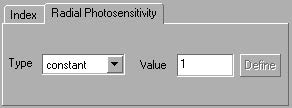
Type
Select one of the following options for the radial photosensitivity profile within the
current region:
Constant – Constant value of radial photosensitivity
Linear
Parabolic
Gaussian
Exponential
Alpha-peak
Alpha-dip
User Function – Functional dependence of the sensitivity, where the function is
defined or programmed using the powerful Script Language environment.
Value
Numerical data entry box – Present when the constant radial photosensitivity option is
selected. Enter the radial photosensitivity value for the selected region. See the
definition of photosensitivity in the technical background section.
Define
Present when the Function or User Function option is selected. Press the Define
button to specify the function. For the built-in functions, a dialog box related to one of
the predefined functions appears. For the User Function option, pressing the Define
button launches the User Defined Function script programming environment.
Azimuthal Photosensitivity
Select one of the following options for the azimuthal radial photosensitivity profile
Constant – Constant value of radial photosensitivity
User Function – Functional dependence of the sensitivity, where the function is defined or programmed using the powerful Script Language environment.
Value – Numerical data entry box – Present when the constant Azimuthal photosensitivity option is selected. Enter the Azimuthal photosensitivity value for the fiber.
Steps – Enter the number of steps for discretization of the Azimuthal photosensitivity
profile user function.
Note: The ‘x” variable in the user defined function is the azimuthal angle from 0
to 2p.
Dispersion Enable
Enable the material dispersion model for the current region. The model definition can
be accessed by pressing the Define button in the Dispersion section of the dialog box
(see Material Dispersion dialog box).
Dispersion Global
Assign the global material dispersion model to the current region. The global model
assumes that a fiber is formed by doping the host material with one dopant that raises
the refractive index and another dopant that lowers the index (see Material Dispersion
dialog box ).
Define Dispersion
Opens the Material Dispersion dialog box, where you can assign a material dispersion
model based on the Sellmeier coefficients library. Alternately you can provide a
custom model.
Real Profile
When the index profile is real, check this check box. Otherwise, uncheck it.
Wavelength
Enter the wavelength in microns. This wavelength is considered as the measurement
wavelength. (The wavelength at which the current profile is exact. For other
wavelength values used in the program (for example when scanning over a spectral
range) the profile shape is adjusted accordingly based on the material dispersion
model, if it is enabled.
Mesh
X: Number of points in the transverse cross-section along the X-axis
Y: Number of points in the transverse cross-section along the Y-axis
The modal fields are calculated based on the mesh setting.
Display
Real – When this radio button is selected, the real index profile will be displayed in the
lefthand display window.
λ – When the Enable check box is checked, enter the wavelength, and the real index
profile at this wavelength will be displayed.
Imag. – When this radio button is selected, the imaginary index profile will be displayed
in the left-hand display window.
PS – When this radio button is selected, the radial photosensitivity profile will be
displayed in the left-hand display window.
Import Profile
Import the real index profile from a text file.
The format of the text file is:
radius in μm refractive index
. .
. .
For example, the text file for a three layers fiber profile is:
4.2 1.451
62.5 1.444
80 1.0
Export Profile
Export the real index profile to a text file
The format of the text file is same as the format described in the Import Profile
Apply
Apply the changes made in the dialog box.
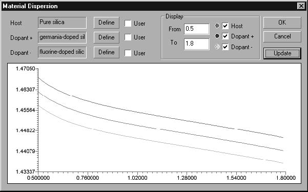
Material Dispersion dialog box
The Material Dispersion dialog box displays the material index as function of
wavelength. For the dispersion model, it is assumed that the fiber profile consists of
regions with only the host material and doped regions. One of the dopants raises the
refractive index, while the other dopant lowers it. The Dopant + and Dopant – curves
show the dispersion curves for materials with a particular kind of dopant (in this case,
Germanium for + and Fluorine for -) at a certain doping concentration. OptiGrating will
use the index given at the centre wavelength in the Single Fiber Profile dialog box to
deduce the concentration in the given layer. With this concentration found,
OptiGrating will interpolate or extrapolate to find the index at other wavelengths. See
the OptiGrating manual, Technical Background chapter for details.
To get the Material Dispersion dialog box:
| 1 | Open the Fiber Profile dialog box. |
| 2 | Select Enable in the Dispersion section. |
| 3 | Press the Define button in the Dispersion section. |
The Material Dispersion dialog box options are described below.
Host
Shows the name of the fiber host material. Press Define to specify the material and
its dispersion model. When the User option is cleared, the Define button activates the
Sellmeier Parameters dialog box. When the User option is checked, the Define button
launches the User Defined Function script programming environment (see the Script
Language section of the documentation).
Dopant +
Shows the name of the fiber material that has higher index due to an index-raising
dopant. The Define button and the User option work the same way as for the Host
option.
Dopant –
Shows the name of the fiber material that has lower index due to an index-decreasing
dopant. The Define button and the User option work the same way as for the Host
option.
Display From
Enter the minimum wavelength for the dispersion display.
Display To
Enter the maximum wavelength for the dispersion display.
Update
Update the dispersion display after recent changes.
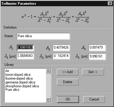
Sellmeier Parameters dialog box
The Sellmeier Parameters dialog box allows you to select the material dispersion
model based on the Sellmeier theory. OptiGrating uses six Sellmeier coefficients,
three wavelengths and three amplitudes, to define the dispersion curve. If the
Sellmeier coefficients for the material at the given doping concentration are known,
you may want to put this in your Sellmeier Coefficient Library so that the dispersion
used lies exactly on one of the curves shown in the Material Dispersion dialog box,
rather than having to rely on an interpolation formula to calculate the effect of material
dispersion. It will also be necessary to add an entry to the library if you are using a
dopant different from the ones already provided.
To access this dialog box, do the following steps:
| 1 | Open the Fiber Profile dialog box. |
| 2 | Select Enable in the Dispersion section. |
| 3 | Press the Define button in the Dispersion section. The Material Dispersion dialog box opens. |
| 4 | In the Material Dispersion dialog box, press the Define button for defining the Host, Dopant +, or Dopant – material model. |
Sellmeier Formula
The Sellmeier formula is displayed for reference. The formula reads:
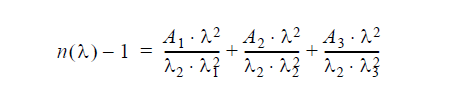
where n is the wavelength-dependent refractive index, λ1, λ2, and λ3 are the
Sellmeier amplitudes, and λ1, λ2, and λ3 are the Sellmeier resonance
wavelengths.
The Sellmeier Parameters dialog box options are described below.
Name
Enter the name of the material. If you select the material from the Library list (see Get
below) then the name appears automatically.
A1, A2, A3
Enter the amplitude Sellmeier coefficients.
λ1, λ2, λ3
Enter the wavelength Sellmeier coefficients.
Add
If you entered new material along with its Sellmeier coefficients, you may add it to the
library by pressing the Add button.
Delete
Delete the selected material from the library.
Get
Get the material from the Library list. The library materials are stored in a data base.
Fiber_CAD provides some of the known materials along with the Sellmeier
coefficients.
Function Definition dialog box
The Function Definition dialog box allows you to define the start and end values in the
current region. The real index profile, imaginary index profile, and radial
photosensitivity use the same set of function definitions.
With this dialog box, you can specify the following predefined functions of the region’s
local radial coordinate x:
Constant index profile:
n(x) = const
Linear index profile:

Parabolic index profile:

Exponential index profile:
![]()
where w is the region width, and n(0), n(w) are the values at x=0 (start) and x=w (end),
respectively. The symbol e denotes the Euler number.
To access this dialog box, do the following steps:
| 1 | Open the Single Fiber Profile dialog box. |
| 2 | Select the Real index list box. |
| 3 | On the list, select Linear, Parabolic, or Exponential. |
| 4 | Press the Define button under the Index option. |
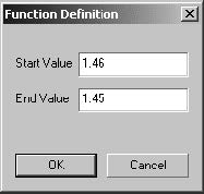
The Function Definition dialog box options are described below.
Start
Enter the start value at the beginning of the region.
End
Enter the end value at the end of the region.
See also the Index Profile of Fibers section in the Technical Background.
Gaussian User Function dialog box
The Gaussian User Function dialog box allows you to specify the Gaussian function
in the current region.
Gaussian profile:
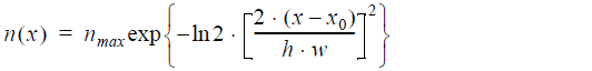
where nmax is the maximum value, x0 is the center (peak) position, and h is the
normalized Full Width at Half Maximum (FWHM).
To access this dialog box, do the following steps:
| 1 | Open the Single Fiber Profile dialog box. |
| 2 | Select the Real index list box. |
| 3 | On the list, select Gaussian. |
| 4 | Press the Define button under the Index option. |
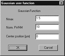
The Gaussian user function dialog box options are described below.
Nmax
Enter the maximum value described by the Gaussian function.
Norm. FWHM
Enter the normalized Full Width at Half Maximum (FWHM) of the Gaussian function.
Center Position
Enter the peak position of the Gaussian function. The position is measured from the
beginning of the current region.
See also the Index Profile of Fibers in the Technical Background.
Alpha Power Law dialog box
The Alpha Power Law dialog box allows you to specify the Alpha-Power function in
the current region. The Alpha-power dependence has two forms: alpha-peak and
alpha dip.
Alpha –peak index profile:
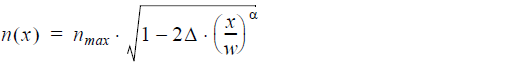
where, nmax is the maximum value and Δ is the normalized difference. It is defined
as
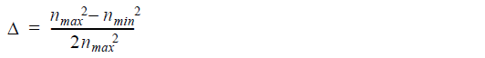
Alpha –dip index profile:

where, nmax is the maximum value and Δ is the normalized difference.
To access this dialog box, do the following steps:
| 1 | Open the Fiber Profile dialog box. |
| 2 | Select the Real index list box. |
| 3 | On the Function list, select Alpha-Power Peak or Alpha-Power Dip. |
| 4 | Press the Define button under the Index option. |
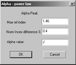
The Alpha Power Law dialog box options are described below.
Max Ref Index
Enter the maximum value described by the Alpha-Power function.
Norm Index Difference %
Enter the normalized difference of the Alpha Power function.
Alpha Value
Enter the alpha power coefficient value.
See also the Index Profile of Fibers section in the Technical Background.
User Defined Function dialog box
The User Defined Function dialog box allows you to specify the user function. The
user defined function can be almost anything that conforms to the rules of the Script
Language programming.
You can find detailed information in the Working With User Defined Options section.
Single Fiber Modes dialog box
After you have finished the data entry in the Single Fiber dialog box, OptiGrating
computes a list of guided modes. This list is displayed in the Single Fiber Modes
dialog box.
Settings
In the Single Fiber modes dialog box, you can define the following options under the
Settings tab:
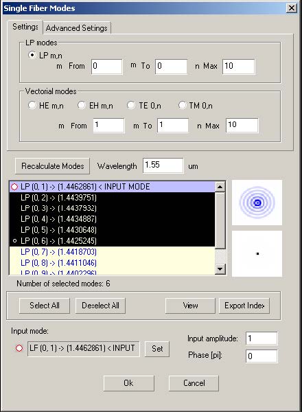
LP Modes
To work with LP modes, click the LPm,n button to enable it and enter the range of the
mode index m (m From to m To) and the maximum value of the mode index n (n Max).
Vectorial modes
To work with vectorial modes, click one of the button (HEm,n EHm,n TE0,n TM0,n) to
enable it and enter the range of the mode index m (m From to m To) and the maximum
value of the mode index n (n Max).
Recalculate Modes
Press this button to start the mode calculation
Select All
Select all the modes from the mode list
Deselect All
Deselect all the modes from the mode list
Set
Set the current selected mode as input mode
Input amplitude
The amplitude of the selected input mode
Phase
The phase of the selected input mode
View
View and export the modal fields. See 3D Preview of the field dialog box.
Export Index
Export the effective refractive index to a text file.
Advanced Settings
Under the Advanced Settings tab, you get the following additional choices:
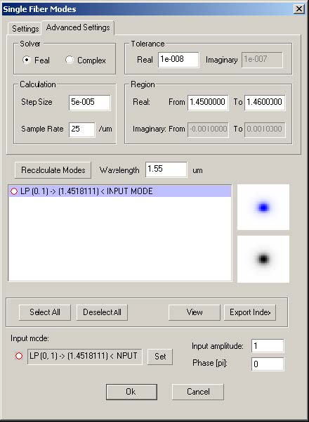
- Choosing Real or Complex will determine which variables you can change.
In the Real option, real solutions will be sought in the interval specified in the Real
From and To fields. The solver will step through this interval in steps of Step Size. In
the Complex option, solutions are sought in a rectangular region of the complex plane
as defined by the From and To fields in both real and imaginary. The Complex option
uses an advanced technique for finding the roots as described in the Technical
Background chapter of the OptiGrating manual.
To compute guided modes
| 1 | File > New. |
| 2 | New > Single Fiber. |
| 3 | In the Project window, click the Fiber/Waveguide Parameters button. |
| 4 | In the Single Fiber Profile dialog box, enter the desired values and press the OK button. |
| 5 | In the Project window, click the Mode Parameters button. |
| 6 | In the Single Fiber Modes dialog box, select modes from the list of guided modes. |
| 7 | In the Input Amplitude and Phase boxes, enter the desired values. |
| 8 | Choose the Advanced Settings tab. |
| 9 | In the Advanced Settings dialog, choose either Real or Complex in the Solver box to enter desired values and press OK. |
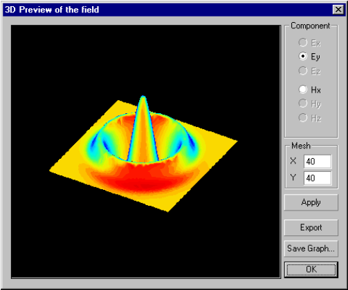
3D Preview of the field dialog box
To Access the 3D Preview of the field dialog box
Follow steps 1 to 5 from the “To compute guided modes” procedure.
| 1 | Press the view button in the Single Fiber Modes dialog box. |
Note: You can also access this dialog box from the Fiber Coupler Modes dialog
box.
The Properties of the dialog box options are described below.
Component
Enable one of the component buttons: Ex, Ey, Ez, Hx, Hy, Hz. The enabled field
component will be displayed and exported.
Mesh
X – Number of points in the transverse cross-section along X-axis
Y – Number of points in the transverse cross-section along Y-axis
Apply
Apply the changes made in the dialog box.
Export
Export the modal field. The file format is the field *.f3d of BPM_CAD.
The exported 3D Complex Format:
BCF3DCX – File Header
NX NY – Number Of x And y Data Points
WX WY – Mesh Width In x And y
Z1 – Complex Number z Data Point With Coordinates (xmin, ymin)
Z2 – Complex Number z Data Point With Coordinates (xmin+dx, ymin)
Z3 – Complex Number z Data Point With Coordinates (xmin+2dx, ymin)
.
ZNX – Complex Number z Data Point With Coordinates (xmax, ymin)
ZNX+1 – Complex Number z Data Point With Coordinates (xmin, ymin+dy)
..
ZN – last Complex Number z Data Point With Coordinates (xmax, ymax), N=NXxNY
Where dx = (xmax-xmin)/(nx-1) and dy = (ymax – ymin)/(ny-1).
Save Graph
Save the graph as a Windows Enhanced Metafile (.emf)
Using Calculation Options
The last step before getting numerical results is to select one of the calculation
options: Propagation, Spectrum, Pulse Response, Parameter Scan.
Propagation
Reflection and transmission along the device.
You can select the number of propagation steps and the signal wavelength. Notice
that the signal wavelength in the Wavelength box can be different from the central
wavelength used in the Single Fiber dialog box. This option allows you to study the
propagation at wavelengths close to the central wavelength. By default, the
wavelength is set equal to the central wavelength.
To use the Propagation calculation option
| 1 | Follow steps 1 to 5 from the “To compute guided modes” procedure. |
| 2 | In the Single Fiber Modes dialog box, select a mode from the list of Fiber Modes. |
| 3 | In the Input Amplitude and Phase boxes, enter the desired values and click the OK button. |
| 4 | In the Project window, choose Propagation from the Calculation list box. |
| 5 | In the Propagation Step box and in the Wavelength box, enter the desired values and click the Calculate button. |
Spectrum
Reflection and transmission at the input and output ports of the device within a range
of wavelengths.
To use the Spectrum calculation option
| 1 | Follow step 1 to 5 from the “To compute guided modes” procedure. |
| 2 | In the Single Fiber Modes dialog box, select a mode from the list of Fiber Modes. |
| 3 | In the Input Amplitude and Phase boxes, enter the desired values and click the OK button. |
| 4 | In the Project window, choose Spectrum from the Calculation list box. |
| 5 | In the From, To, and Step boxes, type the desired values and click the Calculate button. |
Pulse Response
Input pulse intensity spectrum, grating spectrum, output pulse intensity.
To use the Pulse Response calculation option
| 1 | Follow step 1 to 5 from the “To compute guided modes” procedure. |
| 2 | In the Single Fiber Modes dialog box, select a mode from the list of Fiber Modes. |
| 3 | In the Input Amplitude and Phase boxes, enter the desired values and click the OK button. |
| 4 | In the Project window, choose Pulse Response from the Calculation list box. |
| 5 | In the Steps, Time Span, and Wavelength boxes, type the desired values and click the Calculate button. |
To work in the Pulse Response dialog box
| 1 | In the Project window, from the calculation list box, choose Pulse Response. |
| 2 | In the Input View dialog box, click the Define button to open the Pulse Response dialog box. |
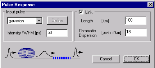
| 3 | In the Input Pulse section, choose either Gaussian or User Defined from the list box. If Gaussian is selected, you will be able to enter an Intensity FWHM value in the Intensity box, where FWHM is the Full Width at Half Maximum in picoseconds. |
| 4 | If you want to define the fiber or waveguide Length and Chromatic Dispersion, enable the Link check box. |
| 5 | The Length is measured in kilometers; the Chromatic Dispersion is measured in picoseconds per nanometer per kilometer. |
Note: If you select User Defined from the list box, the Define button is enabled.
When you click it, you will be able to set your preferences in the User Defined
Function dialog box. If you enable the Link check box, you will see two pulses
displayed in the Input tab of the Project window: the input pulse at the beginning
of the fiber link and the input pulse after propagation through the fiber link, but at
the beginning of the grating.
Parameter Scan
The bandwidth, sidelobe, peak value, peak position and dispersion at central
wavelength within the range of the selected grating parameter. OptiGrating allows you
to define the number of calculation steps.
To use the Parameter Scan calculation option
| 1 | Follow steps 1 to 5 from the “To compute guided modes” procedure. |
| 2 | In the Input Amplitude and Phase boxes, enter the desired values and click the OK button. |
| 3 | From Calculation menu, select Scan. |
| 4 | In the Scan dialog box, type the desired values and click the Calculate button. |
Setting Options in the Fiber Bragg Grating Sensor Dialog Box
The Fiber Bragg Grating Sensor dialog box allows you to set Strain and Temperature
options and to define Strain-optic and Thermo-optic parameters. It is only available
for two layer stepindex fibers.
To define options in the Fiber Bragg Grating Sensor dialog box
| 1 | File > New. |
| 2 | In the New dialog box, click Single Fiber. |
| 3 | From the Parameters drop down menu, click Grating Parameters. |
| 4 | In the Grating Manager dialog box, double-click the desired grating. |
| 5 | In the Grating Definition dialog box, enable the Sensors check box. |
| 6 | Press the Define button to open the Fiber Bragg Gratings Sensor dialog box. |
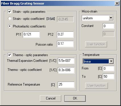
| 7 | In the Fiber Bragg Grating Sensor dialog box, define the Strain-optic and the Thermooptic parameters and the Strain and Temperature options. |
| 8 | Click the OK button. |
Note: For more details about the parameters available in Fiber Bragg Grating
Sensor dialog box, see the Technical Background section.
Setting options in the Long Period Grating Sensor dialog box
In the Long Grating Sensor dialog box, you can define the Strain-optic parameters,
Thermooptic parameters, Cladding, Micro-strain distribution along the grating, and
the temperature distribution along the grating. It is only available for three layer stepindex
fibers.
To define options in the Long Period Grating Sensor box
| 1 | File > New. |
| 2 | In the New dialog box, click Single Fiber. |
| 3 | From the Parameters drop down menu, click the Grating Parameters button. |
| 4 | In the Grating Manager dialog box, double-click the desired grating to open the Grating Definition dialog box. |
| 5 | In the Grating Definition dialog box, enable the Sensors check box and click the Define button to open the Long Period Grating Sensor dialog box. |
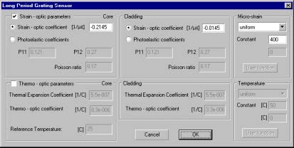
| 6 | In the Micro-strain section, choose one of the following options from the list box: Uniform, Linear, Gaussian, or Used Defined.
|
| 7 | From the Temperature list, choose one of the following options to define the temperature distribution along the grating:Uniform, Linear, Gaussian, or User Defined. |
Note: For information about the Strain-optic Parameters, Cladding, and Thermooptic
Parameters, see the Technical Background chapter.