
In this example, we will simulate a dispersion flattened fiber. We will also demonstrate
the use of the internal scripting language of OptiFiber for defining profiles.
You can find this example as the DFF.fcd file in the Samples directory.
Defining fiber profile
To define a fiber profile, follow these steps:
| Step | Action |
| 1 | From the “File” menu click “New” to open a new project. |
| 2 | Click the “Fiber Profile” icon in the “Navigator” pane. |
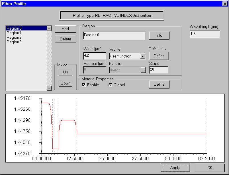
| 3 | Add four regions in the new profile. For “Region 0” enter the following data: Width: 4.2 Profile: user function Click “Define” to enter the script parser editor. In its window enter the following expression: background = 1.4437 delta = 0.01 alpha = 10 background + delta*(1-(x /WIDTH)^alpha) (Thus you defined one half of an “alpha profile” function using the interpreted script language of OptiFiber.) |
| 4 | For “Region 1”, enter the following data: Width: 2.5 Profile: constant Index: 1.4437 Steps: 1 Click “Apply” |
| 5 | For “Region 2”, enter the following data: Width: 6.75 Profile: user function Click “Define” to enter the script parser editor. In its window enter the following expression: background = 1.44692 |
| 6 | For “Region 3”, enter the following data: Width: 49.05 Profile: constant Index: 1.44692 Steps: 1 Click “Apply” |
You fiber profile dialog should look like the one below:
Calculating the characteristics of the dispersion flattened fiber
To calculate the characteristics of the dispersion-flattened fiber, follow these steps:
| Step | Action |
| 1 | Click the “Modes” icon on the “Navigator” pane |
| 2 | Select the “LP Modes” option |
| 3 | Press “Recalculate Modes”. The program provides the modal index at the given wavelength and shows a preview of the modal field. |
| 4 | Click “OK” to leave the “Modes” dialog box. |
| 5 | Click the “Scan Fundamental Mode” icon in the “Navigator” pane. |
| 6 | In the “Properties of Fundamental Mode” dialog box, click “Calculate” to scan the wavelength from 1.3 to 1.8 in 50 steps. |
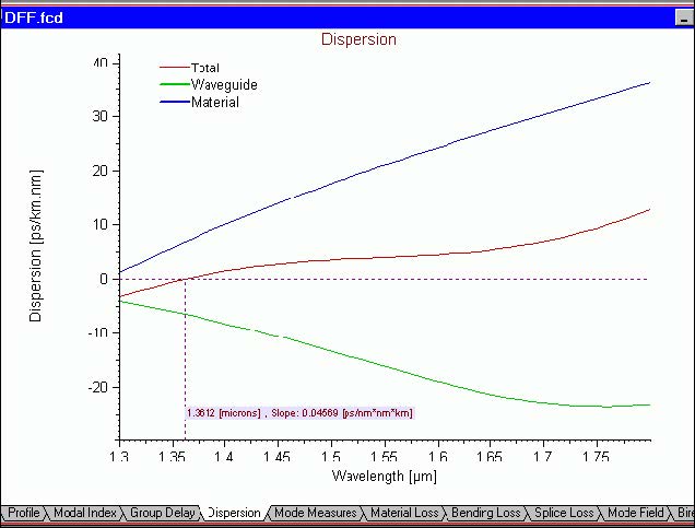
| 7 | Go to “Dispersion” view tab. The total dispersion is small and uniform within the 1.3 – 1.8 ìm wavelength range. |
Your Dispersion view tab should look like this:
You may experiment with scanning some fiber profile parameters, as in “Lesson 3:
Designing Dispersion Shifted Fiber” in order to obtain even better dispersion flatness
or certain value of the average dispersion within a wavelength interval of interest.