
OptiFDTD is a powerful, highly integrated, user-friendly software that allows computer
aided design and simulation of advanced passive photonic components.
The OptiFDTD software package is based on the finite-difference time-domain
(FDTD) method. The FDTD method has been established as a powerful engineering
tool for integrated and diffractive optics device simulations. This is due to its unique
combination of features, such as the ability to model light propagation, scattering and
diffraction, and reflection and polarization effects. It can also model material
anisotropy and dispersion without any pre-assumption of field behavior such as the
slowly varying amplitude approximation. The method allows for the effective and
powerful simulation and analysis of sub-micron devices with very fine structural
details. A sub-micron scale implies a high degree of light confinement and
correspondingly, the large refractive index difference of the materials (mostly
semiconductors) to be used in a typical device design.
2D FDTD Equations
The FDTD approach is based on a direct numerical solution of the time-dependent
Maxwell’s curl equations. The first version of OptiFDTD is in 2D. The photonic device
is laid out in the X-Z plane. The propagation is along Z. The Y-direction is assumed to
be infinite. This assumption removes all the ∂/ ∂y derivatives from Maxwell’s
equations and splits them into two (TE and TM) independent sets of equations.
The 2D computational domain is shown in Figure 1. The space steps in the X and Z
directions are Δx and Δy, respectively. Each mesh point is associated with a specific type of material and contains information about its properties such as refractive index, and dispersion parameters.
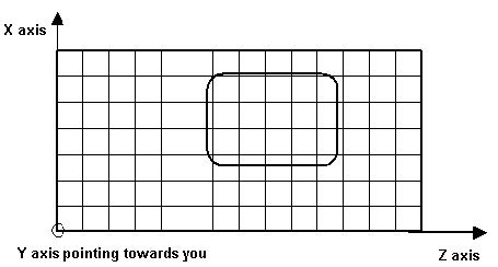
Figure 1: Numerical representation of the 2D computational domain
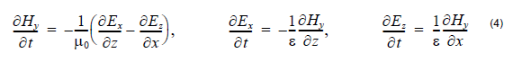
TE waves
In the 2D TE case (Hx, Ey, Hz – nonzero components, propagation along Z, transverse
field variations along X) in lossless media, Maxwell’s equations take the following
form:

where ε = ε0εr is the dielectric permittivity and is the magnetic permeability of
the vacuum. The refractive index is n = √εr.
Each field is represented by a 2D array — Ey(i,k), Hx(i,k) and Hz(i,k) — corresponding
to the 2D mesh grid given in Figure 1. The indices i and k account for the number of
space steps in the X and Z direction, respectively. In the case of TE, the location of
the fields in the mesh is shown in Figure 2.
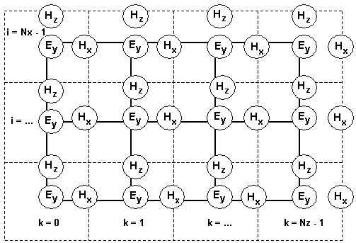
Figure 2: Location of the TE fields in the computational domain
The TE fields stencil can be explained as follows. The Ey field locations coincide with
the mesh nodes given in Figure 1. In Figure 2, the solid lines represent the mesh given
in Figure 1. The Ey field is considered to be the center of the FDTD space cell. The
dashed lines form the FDTD cells. The magnetic fields Hx and Hz are associated with
cell edges. The locations of the electric fields are associated with integer values of the
indices i and k. The Hx field is associated with integer i and (k + 0.5) indices. The Hz
field is associated with (i + 0.5) and integer k indices. The numerical analog in
Equation 1 can be derived from the following relation:

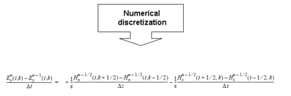
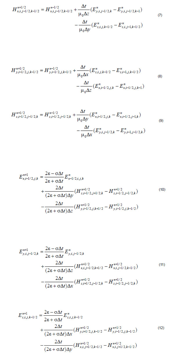
The total set of numerical Equation 1 takes the form:
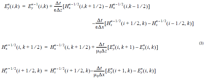
The superscript n labels the time steps while the indices i and k label the space steps and Δx and Δz along the x and z directions, respectively. This is the so-called Yee’s numerical scheme applied to the 2D TE case. It uses central difference approximations for the numerical derivatives in space and time, both having second order accuracy. The sampling in space is on a sub-wavelength scale. Typically, 10 to 20 steps per wavelength are needed. The sampling in time is selected to ensure numerical stability of the algorithm. The time step is determined by the Courant limit:
![]()
TM waves
In the 2D TM case (Ex, Hy, Ez — nonzero components, propagation along Z,
transverse field variations along X) in lossless media, Maxwell’s equations take the
following form:
The location of the TM fields in the computational domain follows the same
philosophy and is shown in Figure 3.
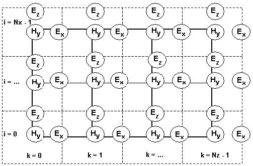
Figure 3: Location of the TM fields in the computational domain
Now, the electric field components Ex and Ez are associated with the cell edges, while
the magnetic field Hy is located at the cell center. The TM algorithm can be presented
in a way similar to Equation 3.
3D FDTD Equations
In 3D simulations, the simulation domain is a cubic box, the space steps are Dx, Dy, and Dz in x, y, and z directions respectively.
Each field components is presented by a 3D array —Ex(i,j,k), Ey(i,j,k), Ez(i,j,k),
Hx(i,j,k), Hy(i,j,k), Hz(i,j,k). The field components position in Yee’s Cell are shown
in Figure 4. These placements and the notation show that the E and H components are interleaved at intervals of 1 ⁄ 2Dh in space and 1 ⁄ 2Dt for the purpose of implementing a leapfrog algorithm.
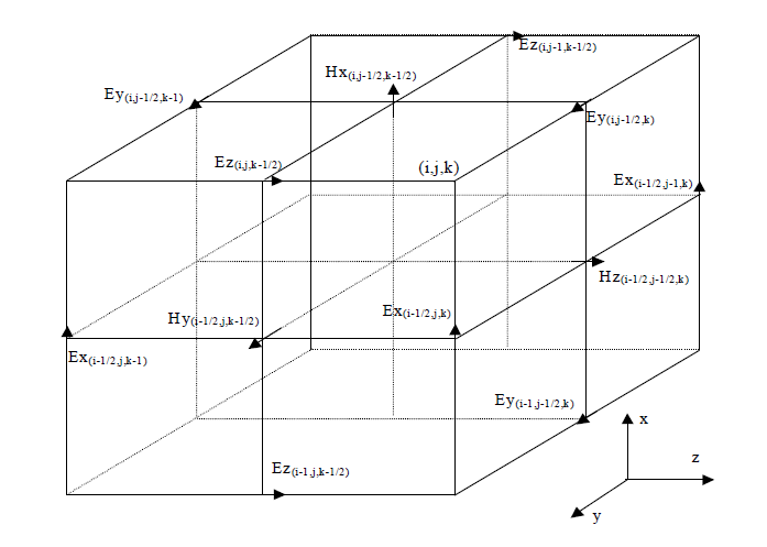
Figure 4: Displacement of the electric and magnetic field vector components about a cubic unit cell of the Yee space lattice
In general, the time domain Maxwell’s equations are given in differential form by
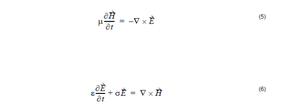
When the second-order finite difference method, field notations, and field
displacements are applied to the above Maxwell’s equation for time domain and
space domain derivatives, the 3D-FDTD formulas can be written as:
Space Step and Time Step
The fundamental constraint of FDTD method is the step size both for the time and space. Space and time steps relate to the accuracy, numerical dispersion, and the stability of the FDTD method. Many references and books have discussed these problems. In general, to keep the results as accurate as possible, with a low numerical dispersion, the mesh size often quoted is “10 cells per wavelength”, meaning that the side of each cell should be 1/10λ or less at the highest frequency (shortest wavelength).
Please note that FDTD is a volumetric computational method, so that if some portion
of the computational space is filled with penetrable material, you must use the
wavelength in the material to determine the maximum cell size.
The following equation is for the suggested mesh size:

where nmax is the maximum refractive index value in the computational domain.
Once the cell size is determined, the maximum size for the time step Δt immediately
follows the Courant-Friedrichs-Levy (CFL) condition.
For 3D FDTD simulation, the CFL condition is:
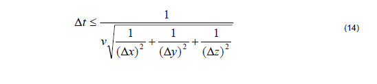
where v is the speed of the light in medium.
OptiFDTD Simulation Procedures
The following is the flow chart for the FDTD simulation in OptiFDTD. It also details the
work flow in OptiFDTD.
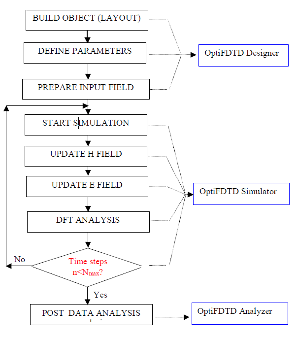
Figure 5: FDTD Simulation Flow Chart in OptiFDTD
Output data
The fields propagated by the FDTD algorithm are the time domain fields. At each
location of the computational domain they have a form similar to that given in Equation
15:
![]()
where B is the amplitude of the field at that particular location, G is the wave profile,
and φi is the corresponding phase. However, the values of B and φi are not
accessible from the time domain field values.
In order to get the full amplitude/phase wave information, we need the stationary
complex fields that correspond to the waveform Equation 15. The complex fields are
the source of all useful information, such as output and reflected powers, overlap
integrals with modal fields, etc. Those complex fields are calculated by a run time
Fourier transform performed in the last time period of the simulation. The final
complex fields can be visualized at specific Output Planes located properly in the
computational domain.
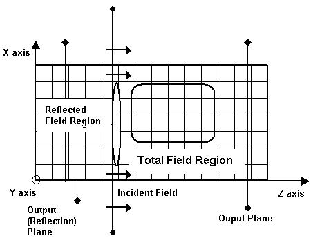
Figure 6: Output Planes
OptiFDTD uses TF/SF (total field/scattering field) technique for the incident plane.
User can specify the incident wave direction. Behind the incident plane, it is the pure
reflection field region, when the observation detectors are placed in this region, the
reflection function can be calculated. When the Observation detectors are placed in
the field transmission region, the transmission function can be calculated.