
Berenger introduced the concept of a perfectly matched layer (PML) for reflectionless
absorption of electromagnetic waves, which can be employed as an alternative to the transparent boundary condition (TBC). The PML approach defines the truncation of the computation domain by layers (which absorb impinging plane waves) without any reflection, irrespective of their frequency and angle of incidence [15] – [18].
PML equations
We consider a 3-D optical waveguide surrounded by PML regions I, II, and III with thickness d as shown in Figure 2. Using the transversely scaled version of PML, Maxwell’s equations can be written as

From Equation 33 and Equation 34 we get:

with
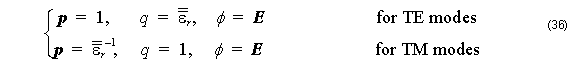
where

Here E and H are the electric and magnetic field vectors, respectively, ω is the angular frequency, ε0 and μ0 are the permittivity and permeability of free space, respectively, n is the refractive index, and σe and σm are the electric and magnetic conductivities of PML, respectively. The modified differential operator ∇’ used in Equation 33 and Equation 34 is defined as
![]()
with

where xˆ , yˆ , and zˆ are the unit vectors in the x , y , and z directions, respectively, and the values of sx are summarized in Table 1.

Figure 2: Optical waveguide surrounded by PML
| Region |
sx |
sy |
| I |
1 |
s |
| II |
s |
1 |
| III |
1 |
1 |
Table 1: Values of sx and sy
The relation in Equation 37 is required to satisfy the PML impedance matching condition

which means that wave impedance of PML medium exactly equals of the adjacent medium with refractive index n in the computation window, ![]() , regardless of the angle of propagation or frequency.
, regardless of the angle of propagation or frequency.
In the PML medium, we assume an m th-power of the electric conductivity as

where ρ is the distance from the beginning of PML. Using the theoretical reflection coefficient R at the interface between the computational window and the PML medium

the maximum conductivity σmax may be determined as

where c is the light velocity of free space.
The parameter s is written as
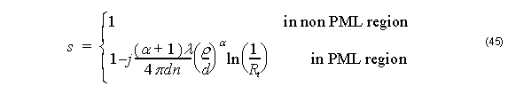
where λ = 2πc ⁄ ω, d, x0, ρ are the free-space wavelength, the PML thickness, the position of the PML surface, and the theoretical reflection coefficient, respectively. Here, the PML is terminated with the perfect electric or magnetic conductor for TE or TM mode, respectively. Usually, a parabolic is assumed for the conductivity, m = 2 .