
We proceed now with the solution of Equation 50 on the basis of the Finite Element Method [29] and [30]. As a first step we introduce the residual

which must be zero in accordance with the state problem. However, it is impractical to enforce R( x ) = 0 at every point in the domain from x = 0 to x = xf . Since φ( xf ) is not expected to vary substantially over a small distance, say Δx , we subdivide the domain into small segments and instead enforce the condition
![]()
over each of the segments. Remarking that Wm ( x ) is some weighting function to be defined later, Equation 84 enforces the differential equation on an average sense over the Ne th segment. By changing the integration or testing interval (and weighting function Wm ) from m = 1 to m = Ne , we can construct Ne equations for the solution of the discretized field values. Before proceeding to do so, we make the following observations about Wm ( x ) :
• If Wm ( x ) = δ( x – xm ) or Wm ( x ) = δ[ x – ( xm + 1 + xm ) ⁄ 2 ] the resulting weighted residual procedure is referred to as point matching and leads to a form of the finite difference method.
• If Wm ( x ) is set equal to the basis functions used for the representation of φ( x ) , the procedure is referred to as Galerkin’s method. This is the most popular testing/weighting method for casting the differential equation to a linear system.
• The choice of Wm ( x ) is not completely arbitrary. For the mathematical steps in the FEM procedure to hold rigorously, Wm ( x ) and its derivative must be at least square integrable over the domain. Specifically, for the problem at hand, it must satisfy the condition

In addition, Wm ( x ) must satisfy conditions at the boundary nodes (end-points at x = 0 and x = xm ) for the one-dimensional problem which are compatible with the imposed boundary conditions. Certain smoothness conditions on Wm ( x ) and ![]() may also need to be imposed.
may also need to be imposed.
Before generating a linear of equations from Equation 84 subject to the boundary conditions, it is first necessary to cast in a more suitable form by following the steps:
Step 1: Take advantage of the weighting Wm ( x ) to reduce the order of the derivatives contained in R( x ) . To do so we employ integration by parts, giving:
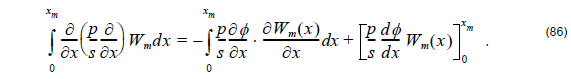
The last right hand side term can be evaluated by enforcing the known boundary conditions at the endpoints. Its effect on the overall system will be considered later.
Step 2: Derive the “weak form” of the differential equation. The weak form of the differential equation is most appropriate for numerical solution and is obtained by substituting Equation 86 into Equation 84.
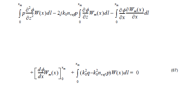
which holds providing Equation 50 is valid. However, because of the integral, the weak form Equation 87 enforces the differential equation on an average (and therefore weaker) sense.
a) Discretization of the “weak” differential equation
The discretization of Equation 87 to a linear set of equation is done by introducing an expansion for φ( x ) and then making appropriate choices for the weighting functions. We chose the linear representation

where φej ( x ) are the unknown coefficients of the expansion. When eo = 2 , we define linear elements. In this case, the basis functions for element e are defined as


Figure 5: Nodal expansion function for eth functions considering linear approximation
The basis functions have unit magnitude at one node and vanish at all others with linear variation between the nodes. When eo = 3 , we have quadratic elements that are also known as second order elements. Each element has three nodes, one of two endpoints, and the third is usually placed at the center of the element. Within each element, the unknown function is approximated as a quadratic function
![]()
Enforcing Equation 91 at the three nodes of the element yields:
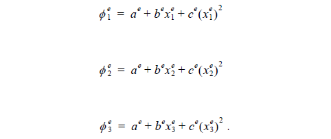
Solving for ae, be, and ce and substituting them back into Equation 91, we obtain

where the interpolation or expansion functions are given by
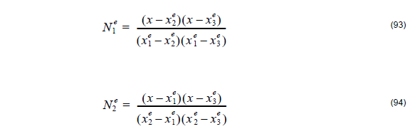

 Figure 6: The nodal expansion function for eth functions considering quadratic approximation
When the expansion Equation 92 is substituted into Equation 87 we get
The terms in the brackets are due to contributions from endpoints of the domain and their evaluation is subject to the specific boundary conditions. This equation now explicitly shows how the boundary conditions enter into the construction of the linear system. Hereon, we will refer to their contributions as endpoints since we have not yet specified the type of boundary condition to be imposed.
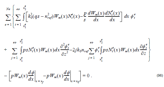
We are now ready to make different choices for the weighting function to generate a system of linear equations for the solution of { φ n} . As stated earlier, this step is also referred to as testing and Galerkin’s method is usually employed in the finite element method. Specifically, we choose Wm ( x ) = Nje ( x ) and for each of these testing or weighting functions a single linear equation is generated.
From Equation 96 we have
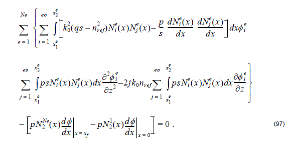
We can rewrite Equation 97 in matrix form as
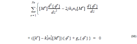
where { φe } is the element electric or magnetic field, { 0 } is a null vector and the element matrices [ Ke ]ij and [ Me ]ij are given by
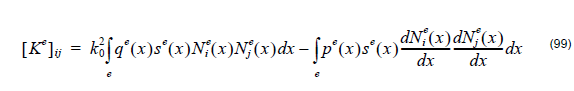
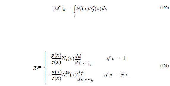
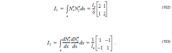
Here [ Ke ]ij and [ Me ]ij are tridiagonal when we use linear base function to expand the field element or pentadiagonal when we adopt quadratic base function to expand the field. Since Nie ( x ) are linear functions, the evaluation of integrals can be carried out in closed form provided pe(x) and qe(x) are taken as constant over integration of the eth element. Specifically, setting pe ( x ) ≅ pe and qe ( x ) ≅ qe for xle < x < x2e .
As a result of integral evaluation we have
(1) Linear elements:
(2) Quadratic elements:


Here le = x2e – x1e.
b) Boundary Condition
The endpoint contributions appear only when e = 1 or e = m and vanish when the Neumann

or Dirichlet conditions φ|x = 0 = φ| x = xf are imposed.
To set the TBC as defined in “Transparent Boundary Condition” on page 23, we
define:

Here,

where the real parts of k1, i and km, i must be restricted to be positive to ensure only radiation outflow.
For Dirichlet, Neumann, and TBC boundary conditions, we set s = 1 . For PML, we introduce the parameter s as defined by Equation 45.