
In actual structures, radiated waves are reflected at the boundaries and return to the core area, where they interact with the propagating fields. This interaction disturbs the propagating fields and greatly degrades the calculation accuracy. It is usual to impose boundary conditions when formulating propagation algorithms in such way to avoid radiation from the device to be reflected at the boundaries, which could couple back into guided modes of the device. These mentioned reflected waves from the boundaries could cause significant errors, particularly if these boundaries are not far enough away from the waveguide. Therefore, one of the key issues in implementing BPM code to study light propagation in a finite spatial domain is the boundary condition at the computation window edges.
The conventional approach is to use an Absorbing Boundary Condition (ABC) in which an artificial layer of lossy material is placed around the computational window. However, to efficiently absorb any outward going radiation with as little reflection as possible, requires careful tailoring of this absorbing region to determine its optimum thickness and absorption coefficient. Therefore, application of the ABC requires additional resources in computational time and memory. Another technique is the Transparent Boundary Condition (TBC) where an absorber is not used but the field is assumed to behave exponentially near the boundary [10], [11]. The TBC is far more economical than the ABC as it contains no adjustable parameters and is therefore more robust. More recently, the Perfectly Matched Layer (PML) boundary condition has been proposed which relies on the anisotropic properties in conductance of a non-physical medium surrounding the problem space. Suitable choice chose of these conductivities ensures very small reflections from the boundary [12].
The Transparent Boundary Conditions (TBC) and the Perfectly Matched Layer (PML) are the most effective way to handle strong radiation at the boundaries [13].
Transparent Boundary Condition
TBC is a boundary condition that simulates a nonexistent boundary. Radiation is allowed to freely escape the problem without appreciable reflection, whereas radiation flux back into the problem region is prevented.
The Transparent boundary condition (TBC) is obtained by assuming that the field in the vicinity of the virtual boundary consists of an outgoing plane wave and does not include the reflected wave from the virtual boundary. Then we assume that the wave function for the left-traveling wave with the x -directed wave number kx is expressed as
![]()
As can been seen in Figure 1, denote the x coordinates and electric fields of the nodes at
p = –1, 0, 1 as x–1, x0, x1 and as φ–1 , φ0 , φ1 . Assuming Equation 25 for each mesh point we can get:

where Δx = x2 – x1 = x0 – x–1 .
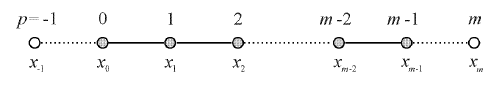
Figure 1: Nodes p = –1 and p = m are outside the analysis domain
From Equation 26 we can derive the -directed wave number:
![]()
If the real part of kx is positive, then the plane wave expressed by Equation 25 propagates toward the outside of the boundary. If the real part of kx , Re( kx ) , is negative, the plane wave of Equation 25 propagates toward the inside of the boundary. When we are dealing with a waveguiding structure that has no reflecting element, an inward-propagating wave should not exist. Therefore, in such a case Re( kx ) must be made positive:
![]()
The wave number of the outgoing plane wave at the right-hand boundary is obtained
in a similar manner. Then we assume that the wave function for the right-traveling wave with the x -directed wave number kx is expressed as
![]()
As can been seen in Figure 1, let denote the x coordinates and fields of the nodes at as
xm – 2, xm – 1, xm , and as φm – 2, φm – 1, φm .
Assuming Equation 29 for each mesh point we can get:

![]()
where Δx= xm – 1 – xm – 2 = xm – xm – 1 .
From Equation 29 or Equation 30 we can derive the x -directed wave number:
![]()
Similar to the left-hand boundary case the real part of kx , Re( kx ) , must be restricted to be positive to ensure only radiation outflow. When it is negative, which implies reflection occurs at the right-hand boundary, the sign should be changed from minus to plus.
As can been seen, the beam propagation including a radiation wave can be analyzed easily and efficiently by using the above-mentioned transparent boundary condition. The fundamental aspect of the TBC method is the plane-wave approximation of the radiation wave and the successive renewal of the wave number kx by using the former step-field distribution [14].