Loading [MathJax]/extensions/tex2jax.js

Lesson 6 – Reconstruction of Unknown Grating

Home » Blog » Lesson 6 – Reconstruction of Unknown Grating

In this lesson we check that the layer peeling algorithm can reconstruct an unknown
grating with knowledge of only the reflection coefficient. In the first step, we select a
typical grating with chirp and apodization and calculate its reflection coefficient. This
spectrum is then exported to a text file. In the next step, OptiGrating is run again and
the spectrum file imported. The layer peeling algorithm is applied to the imported
spectrum to reconstruct the original grating.

Step
1	File > Open. Choose file Ex1a.ifo.
2	Select the Profile tab to see the details of this grating.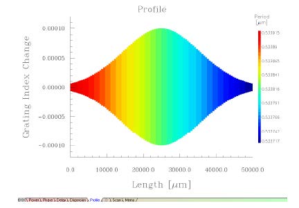 It has a linear chirp of 0.2 nm, and a gaussian apodization with FWHM = 0.5.
3	Select the Power tab to see the reflection and transmission spectra.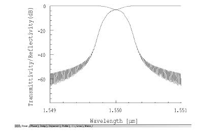 Note: You can press Calculate to calculate the spectrum again, if desired.
4	Click on Spectrum in the Single Fiber drop down menu, then click on the graph in the main window to active it.
5	Select Tools > Export Complex Spectrum and select the Reflection button as shown below: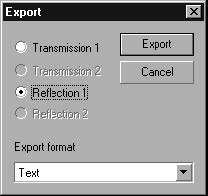
6	Click Export.
7	In the Save As dialog box, find a suitable place and name for your data file.
8	Close Ex1a.ifo.

Step
1	Now, open a new project with File > New > Single Fiber.
2	Choose Calculation > Inverse Scattering Solver to get the Inverse Problem Solver dialog box.
3	Select the From File checkbox.
4	Navigate to the place where you left the file with the reflection spectrum. Open the file.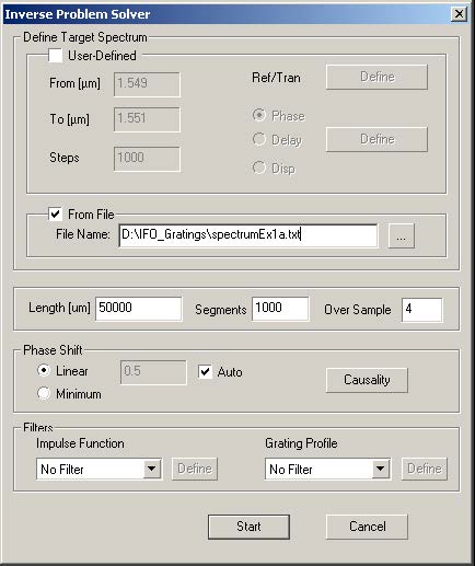
5	We suppose that the original length of the grating is known, so enter 50000 μm in the Length box. (Feel free to experiment with different lengths.) The original spectrum was generated with a profile having 100 segments. It is not necessary that the reconstruction have the same number, here it is set to 1000.
6	Click on the Causality button to test this spectrum.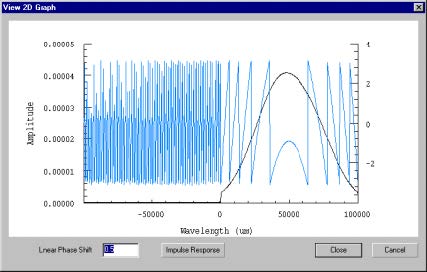 Since this spectrum was generated from a real grating, it displays exactly the causal property of being zero for negative argument.
7	Click Close.
8	Click Start in the Inverse Problem Solver dialog box to begin the reconstruction.
9	Click on Spectrum to enable all tabs.
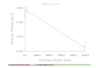
10	Select the Profile tab to see the reconstructed profile.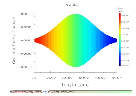 The apodization appears to be a similar shape as the original grating.
11	To see the chirp more clearly, right click the mouse in the Profile window and select Chirp Period.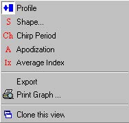 . . . to get the following: The chirp is linear and shifts by 0.2 nm, like the original grating.
12	Select the Power tab to compare the reflectivities, one from the imported complex spectrum and the other from the calculated response of the reconstructed grating.