
![]()
OptiSPICE 5.3 introduces several enhancements including new models and devices, improvements to the simulator performance & post processing features, and a major visualization update.
Key new features include:
- New Probe Visualizer that enables users to view simulation results directly from the schematic (as an alternative to using OptiSPICE’s waveform viewer).
- Enhanced Simulation Engine. Improvements include: Enhancements to the sparse matrix solver libraries; Updates to UMFPACK and MKL for improved stability; Ability to control time step sizes during parameter sweeps (engine uses an improved initial guess for DC sweep, transient and operating point simulations).
- Improved Optical S-Parameter model which now supports time delay. The value for the time delay can be specified by the user or calculated from S-Parameter data. The S-Parameter model has the ability to simulate passive optical devices characterized by different methods (such as OptiFDTD/OptiBPM simulations and experimental results).
- Replacement of optical signal labels “forward” and “reverse” to improve user experience when analyzing simulation results. Optical signals are now labeled “input” and “output”.
Visualization and Post Processing Enhancements
New Probe Visualizer
A new probe, called Probe Visualizer, has been added to OptiSPICE’s device library. This new visualizer can be placed anywhere in the circuit like a regular probe. It has been implemented to help users evaluate the simulation results and debug circuits without exiting the circuit schematic. Once simulations complete, users can simply double-click the probe visualizer to view the results.
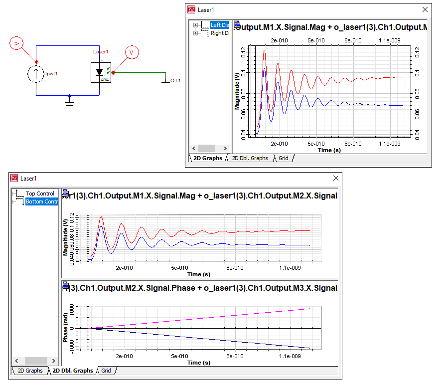
Fig. 1 – This example shows the plotting of the laser turn-on transient at different frequencies. The new probe visualizer allows users to view results directly from the schematic.
Simulation Engine Improvements
A wide range of improvements have been made to the simulation engine. The 3rd party sparse matrix solvers, UMFPACK, and MKL have all been upgraded to newer versions for improved stability and convergence. The simulation engine has also been configured to allow user controlled time steps for transient parameter sweep simulations.
![]()
Fig. 2 – Transient parameter sweep simulations can now be setup with user defined minimum and maximum time steps. The figure above shows the step response of an RLC filter where resistance is swept between 0.5 and 5 ohms and the time step is set to 1 ps.
Updated Optical S-Parameter
A new Optical S-Parameter component with enhanced features has been added to the OptiSPICE library. It can accept measured or simulated S-Parameter files in Touchstone format. It also supports different time delays on each S-Parameter, which can be user defined or calculated from the phase. In addition, the S-Parameter component now has improved stability, accuracy and convergence.
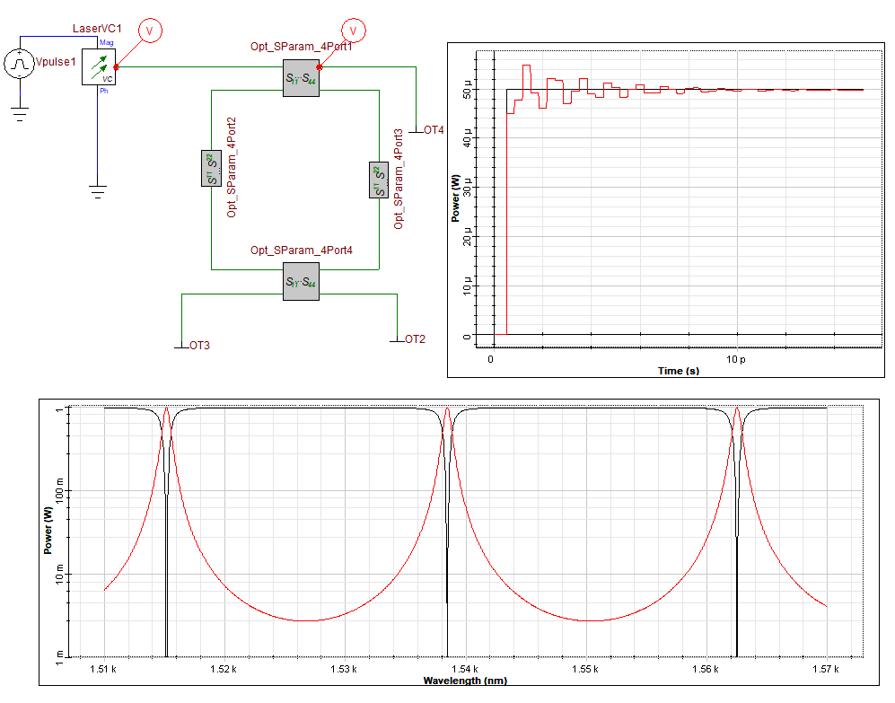
Fig. 3 – The example above shows a ring resonator simulation using only S-Parameter components. The graph on the right shows the step response of the ring resonator as the input travels along the ring and interferes with itself. The bottom graph shows the frequency response of the ring resonator’s through and drop ports.
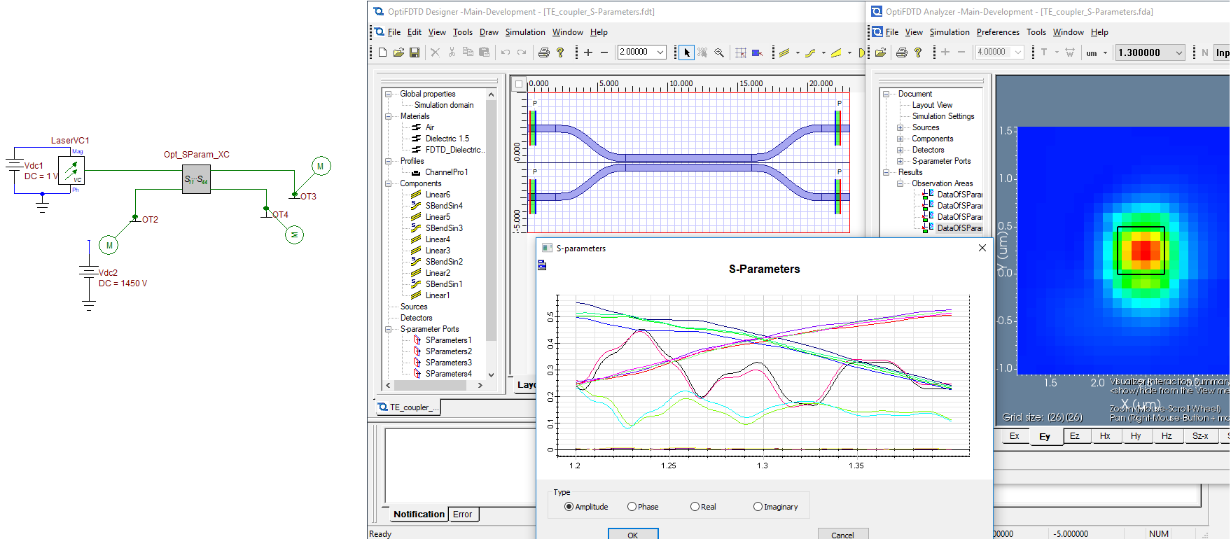
OptiSPICE’s S-Parameter component accepts S-Parameters extracted by OptiFDTD and OptiBPM simulations. OptiFDTD and OptiBPM can be used to characterize passive optical components, and then pass that data into OptiSPICE for photonic circuit and system simulation.
Optical Output Labels
The naming convention for the optical signal labels has been changed to help users easily identify various optical signals entering and leaving optical devices in the schematic. “Reverse” and “forward” labels have been completely removed. Optical signals leaving an optical device are now labeled “output” and optical signals entering an optical device are now labeled “input”.
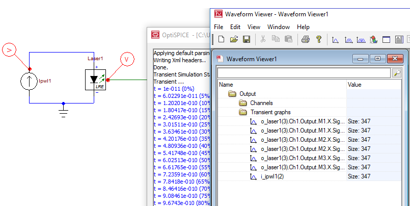
Fig. 4 – The example above shows the output of a multimode laser with different frequencies.