
This lesson demonstrates the average soliton regime at 10 Gb/s transmission over a 500 km optical link consisting of SMF.
Figure 1 shows the layout that was used.

Figure 1: Average soliton regime layout
Figure 2 shows the global and pulse parameters used to achieve transmission at 10 Gb/s.


Figure 2: Simulation and Main parameters for 10 GB/s transmission
We fixed B = 10 Gb/s → TB = 100 ps.
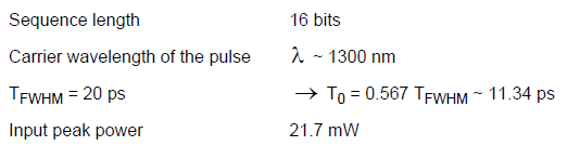
Figure 3 and Figure 4 show the selected parameters.

Figure 3: Fixing Nonlinear Dispersive Fiber Main parameters

Figure 4: Fixing Nonlinear Dispersive Fiber Dispersions parameters
We will consider SMF with a length of 50 km and losses of 0.4 dB/km.

Note: The effects of group delay and third order of dispersion are not taken into account.
After each fiber, the signal is amplified with SOA. Therefore, LA ~ 50 km. Note that the condition LA < LD is satisfied (see Figure 5).

Figure 5: Nonlinear Dispersive Fiber Nonlinearities parameters
The Kerr nonlinearity coefficient y = n2ω0/cAeff for the fixed values of nonlinear refractive index n2 = 2.6 10-20 [m2/W],
![]()
The linear losses for 50 km SMF are 20 dB. The losses are periodically compensated with the Ideal EDFA with 20 dB gain.
Soliton peak power for this SMF is 5.8 mW. The input power of the average soliton is 27.1 mW. To demonstrate the importance of the input power of the average soliton, we will consider soliton propagation in a 500 km SMF with two different input powers:
5.8 mW — usual soliton peak power (Version insufficient power)
27.1 mW — modified soliton peak power which takes into account the periodical amplification (Version average soliton)
Each version includes sweeps on the number of loops 0, 4, 7, and 10 with which to represent the propagation distances 0, 200, 350, and 500 km in SMF.
Figure 6 shows the initial pattern of pulses, and the same pattern of pulses after 200, 350, and 500 km transmission in SMF and periodic amplification with EDFA at every 50 km with the 27.1mW — modified soliton peak power which takes into account the periodical amplification.

Figure 6: Average soliton pulse patterns
Good preservation of the pattern of pulses can be clearly seen. The average soliton concept is valid for these pulse, fiber, and amplification parameters.
Figure 7 shows the initial pattern of pulses, and the same pattern of pulses after 200, 350, and 500 km transmission in SMF and periodic amplification with EDFA at every 50 km with the 5.8 mW — soliton peak power which doesn’t take into account the periodical amplification.

Figure 7: Insufficient power pulse patterns
Because of the improper pulse power used, the pulses in the pattern do not preserve their forms. As a result, pulses broaden and complicated structures appear.
This lesson demonstrated the average soliton concept. It requires:
- fulfilment of adiabatic condition LA < LD
- proper pulse peak power which to take into account the process of periodical amplification
References:
[1] G.P. Agrawal, “Applications of Nonlinear Fiber Optics”, Academic Press, 2001.
[2] G.P. Agrawal, “Fiber Optic Communication Systems”, 2nd Edition, John Wiley & Sons Inc., 1997.