
In order to reduce the partial differential equation into difference equations for solving,
a mesh needs to be defined and applied. The mesh used is shown in Fig. 1 below. It shows a sample of the mesh at a point P that is not on one of the calculation window boundaries. The magnetic fields are defined at the nodes (dots at the intersections), and the permittivity is defined in the rectangular regions bounded by the nodes. The permittivity inside the rectangular regions εNE , εNW , εSE , and εSW is taken to be constant, so inside each of these regions, the equations (8) and (9) apply.

Figure 1: Mesh for the finite difference equation. The magnetic field is defined at points N, S, E, W, and P. The permittivity is defined in the rectangular regions bounded by the nodes.
The mesh is in the transverse plane, and (8) and (9) do not, by themselves, introduce coupling between the field components hx ( x, y ) and hy ( x, y ) . The coupling comes from matching the transverse components of electric and magnetic fields at the boundaries.
In Ref [1], the magnetic fields inside the rectangular regions are expanded to the second order in derivatives defined at the centre point, P. Those expansions are used to estimate what the longitudinal components ez and hz will be at the horizontal and vertical boundaries between the points N, S, E, W, and P. Once this is done, an equation involving the magnetic field components at the nodes is eventually obtained:
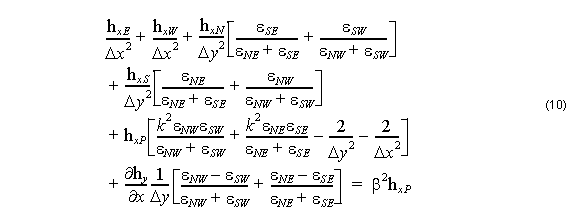
Equation (10) comes mostly from (8) for hx . In the matching of transverse components of the fields, another term involving hy appears. This is the term that is responsible for the coupling of hx and hy . In the finished finite difference formulation, the derivative of hy with respect to x is replaced by a centred finite difference. Note that if at this particular node, it happens that the permittivity is the same on the north side of the boundary as on the south (i.e. it is a vertical boundary), no coupling will occur, or at least there will be no contribution from the of this node. hy component This equation (and a similar one for hy ) is applied to each node in the mesh. Let the number of nodes be n. It is the repeated application of this equation, and the adjustment of the meaning of the N, S, W, E, and P designations, that generates a large system of linear equations. The values of the x and y components of the magnetic field are collected in a vector of dimension n x 1, called v , say. The equations on the left form an n x n matrix Q that multiplies v , and the right hand side has the original vector representing the magnetic field, multiplied by the eigenvalue β2 . In vector-matrix form, the problem looks like
![]()
and to find the modal indices ( nmod = a classical eigenvector problem. β ⁄ k ) and modes, v , is a matter of solving