
The realistic layout of the “mux/demux” example in OptiBPM looks as shown in
Figure 8 (note the size ratio of 1:10). What first attracts our attention is the presence of a
number of relatively primitive, i.e. straight and curved, waveguides. The layout is very coarse compared to the entire wafer area. Moreover, the light interactions actually occur on just a small fraction of the layout. In addition, all six four-port couplers are identical (see Figure 9).

Figure 8: Mach-Zehnder MUX/DEMUX example in OptiBPM—Size ratio 1:10
Let us mark the couplers as shown in Figure 9. At this point we encounter the key point of the approach – its division criteria with the respect to the sub-circuit functionality. We have to split the circuit into the particular cells. The cells must be self existing fully functional units, although the splitting of the whole device must not disturb its functionality in any way when later composed together by means of the OptiSystem.

Figure 9: Six identical couplers
This may be recognized as a weak point of the presented method, everything depends on skills and experience of the user. On the other hand, the subunits mostly appear naturally from the basic design. This fact reduces the possibility of error.
It is obvious, we can pick the six couplers off the layout to simulate (and/or optimize or slightly modify) just one (the four port coupler is shown in Figure 10), later applying six times the obtained result.

Figure 10: Four-port coupler
We have the number of remaining single waveguides to describe. We can do so in several possible ways and we may recognize another step of flexibility of the method.
First the most accurate way is to simulate them by BPM similarly to the coupler – let us call it total analysis with respect to this approach. However, the detailed study is not needed for all waveguides. We would prefer to do so for the waveguides playing a role between the couplers, since we are primarily interested in the phase difference between the arms. The waveguides connecting the ports with the “core” of the device (i.e. the outermost waveguides) are simple isolated waveguides engaged in modal propagation in the fundamental mode. After some preliminary inspection we can even neglect the losses or we can prescribe them analytically. In other words, a user’s experience and intuitive estimation says how far any approximation may be used. This means we can approximately assume the power overlap integral to be the unity at the end of the waveguide and we have to find the phase delay according to Equation 4. The style of the S-data file is obvious. To generate these data analytically requests only the knowledge of the propagation length(s) and the modal indices. This can be even done by any spreadsheet codes. We will also supply a user with a short engine creating the files soon. The huge advantage here is we do not employ any numerical technique to describe all the waveguides where numeric yields no essential results. Short inspection apparently shows the power overlap integral differs by negligible amount after relatively long propagation in the straight waveguide. We thus need to consider the phase delay, as described above.
What about the efficiency of the method? We can see we have to run the BPM for only small fractions of the whole layout. This saves an immense portion of the simulation time and we are missing no essential information about the light traveling on the layout. To be more specific, let us show the final design of the mux/demux device in the OptiSystem environment.

Figure 11: Remaining primitive waveguides from layout
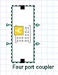 The four-port coupler takes the form shown on the left. The icon possesses all the desired data with respect to the power transfer, the phase delay as the dependencies on the considered wavelength interval.
The schematic representation of the device according to the original schematics is shown in Figure 12. For an example, note the direct (analytical) connection from the coupler ‘b’ to the output A, because there is no special functionality of that upper waveguide. Introducing the light sources and the analyzers (power meters), we may run the simulation. Since we are dealing with small matrices, the simulation takes only negligible time.

Figure 12: Four-port coupler schematic in OptiSystem environment
Figure 13 details the flexibility of the OptiSystem tool. If there is no need for the exact analysis, we can skip some numerical simulations and simulate only those parts we are interested in. The simplest layout is shown in Figure 13.

Figure 13: OptiSystem simple layout
We have numerically studied only the phase differences of each arm, and we exploited analytically prescribed 3dB coupler. We may exchange any S-data part of the simulation by an analytical model and vice versa. This possibility opens very huge field for the additional study of a device, its modification, pre-calculation, partial analysis (e.g. one can put the power meter in any suitable place inside the layout) and many others. You can see the agreement with the original paper [5] (we show only one channel signal for the sake of brevity). The files are available in the template library of Optiwave products.
")
Figure 14: Power vs. Frequency dependence (at port ‘C’)