Fiber Mode Solvers

Introduction

Many kinds of optical fiber can be described, or in the case of graded index fibers,
approximated by, a series of concentric layers of loss-less dielectric. When the index
contrast in the structure is small, it is common to use the scalar wave equation to
obtain the linearly-polarized modes (LP modes). However, when the index contrast
becomes larger, the LP approximation becomes inaccurate, and a full vector analysis
is necessary [1]. Within any one of the concentric layers, the field components are all
linear combinations of Ordinary and Modified Bessel functions, and the solution is a
matter of matching the tangential field components of adjacent layers, leading to the
solution of a linear system. There are some choices to make about the best way to
arrange the linear system (see Ref. [2] for a complete treatment) but probably the best
choice for a general, quick algorithm is the method of Yeh and Lindgren [3]. The
method has intuitive appeal in its similarity to the transfer matrix method used for the
analysis of planar waveguides [4]. Both methods use a matrix to express the fields at
one side of a layer given their values at the other side, and the whole structure is then
characterized by cascading the layers by matrix multiplication. For vector fields in
fibers, there is no natural separation into TE and TM polarization, so one must include
the two tangential components for both electric and magnetic field simultaneously. In
total there are four transverse components at the layer boundaries, so the transfer
matrix in fiber is a 4×4 matrix, instead of 2×2.

The method used by the Optiwave fiber mode solvers is different from the previous
works in three ways. The 4×4 matrix method for vector modes in fibers is
implemented with these improvements to make the algorithm faster in execution time,
and more reliable in the finding of modes, particularly in cases where the modes are
almost degenerate. The first improvement involves a reformulation of the basic
equations to make a real-valued numerical implementation. Since it is loss-less
modes on a fiber of loss-less material that is being sought, there is no reason to
include complex numbers in the formulation. Real-valued implementation uses less
computer resources. Second, the complete transfer across one layer boundary
requires a matrix inverse. It is better to find this inverse analytically, rather than rely
on numerical inversion at each stage. The layer matrix can be decomposed into two
4×4 matrices, and the new matrices are of a form where it is easy to find the inverse
by inspection, thereby finding the analytic solution to the original inversion problem.
Third, it is usual to construct the dispersion function (the zeros of which are located at
the modal indices) as the determinant of the 4×4 matrix system. While this is
theoretically correct, it is not the most intuitive prescription. Worse, the determinant is not the most convenient construction for locating the zeros, particularly in the case
where two zeros are very close to each other. Optiwave uses an eigen-value analysis
that splits the dispersion function into two functions. This splitting resolves the almost
degenerate pairs and helps the simple-minded computer algorithms to find the zeros
of the dispersion function (i.e. the modes) more reliably.

Real-valued formulation

The time independent Maxwell curl equations with a positive time convention ( e^jωt ) are

and the divergence equations are

The factor j does not suit the current purpose, so make the substitution

where  is the free space impedance, so that h and E have the same
units. Then

where . Eliminating the h gives the electric wave equation

Debye Potential

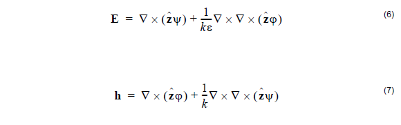
For finding electromagnetic fields in a cylindrical geometry it is convenient to use
cylindrical coordinates r, θ and z, and Debye potentials parallel to the axis of rotation, [2]

It is supposed that the permittivity is constant in the region in which the above
equations apply. The fibers are defined as a series of concentric layers of constant
dielectric, so for the fiber mode solver, the region is the annulus between the layer
boundaries. Equation 6 and Equation 7 are applied in a piecemeal way. Strictly
speaking, the ψ, φ and ε should have subscripts to indicate to which layer the
solution applies, but they are dropped here to simplify the representation. The
complete solution for the multilayer fiber will be constructed by using a separate pair
of functions for each layer, and by matching the tangential field components at the
layer boundaries

The divergence of the curl of any vector field is identically zero. Therefore the choice
of (6) and (7) to represent the electric and magnetic fields means that the divergence
equations (2) will automatically be satisfied. In the remainder of this section, we show
that if the two potentials ψ and φ are solutions to the scalar Helmholtz equation, then
(6) will be a solution to the Maxwell wave equation (5), at least within any given layer.
In subsequent sections, the particular solution for the mode will be found by observing
the boundary conditions imposed by physical considerations on E and h.

Suppose ψ is a continuous function of position that satisfies the Helmholtz equation
in 3 dimensions

Consider the following equation, true for any ψ satisfying (9) in a region of constant
permittivity.

Associate the first two terms together and apply the vector identity

to get

The right hand side of (11) is a gradient of a scalar function, so the curl of the left hand
side must be zero. take the curl of (11)

and define E by the first term of (6). With E defined this way, the Maxwell electric
wave equation (5) follows, and therefore this E is a possible solution for electric field.

Solutions defined from the Ψ function solely (that is to say, solutions with φ = 0), will
have electric fields of the form

from which we can see there is no longitudinal (z) component to the electric field, i.e.
these are transverse electric fields. The magnetic field associated with these
transverse electric fields is constructed from the first Maxwell curl equation in (4):

which is the second term of (7).

The same sequence (7) – (11) can be applied to the φ function to give transverse
magnetic fields, and the electric components of these are given as the second term
of (6). A linear superposition of transverse magnetic and transverse electric fields will
give solutions that are neither transverse magnetic nor transverse electric. In fact,
most modes of the fiber are of this hybrid kind. In the hybrid case, equations (6) and
(7) are used as written, and the relative value of the ψ and φ is now important, since
it is a specific linear combination that matches the boundary conditions at the layer
boundaries.

Separation of Variables

The potentials themselves are solutions of the scalar Helmholtz equation, and the
particular solution is found by observing the boundary conditions imposed by physical
considerations on E and h. The potentials are supposed to form modes, so a solution
where the variables are separated is appropriate

and a similar expression applies for the other Debye potential, φ . The Helmholtz
equation (8) is expanded in cylindrical co-ordinates, and then (15) is substituted.For
regions where ε is constant, the radial functions follow the Ordinary or Modified
Bessel equation, and so the solutions are linear combinations of Bessel functions of
integer order v. In any given layer,

where . In layers where the propagation constant squared is
larger than k²ε, the Bessel functions J and Y are replaced by the Modified Bessel
functions I and K, respectively.,

where . Equations (15), (16), and (17) are substituted in (6) and (7)
to find the electromagnetic fields. It is the tangential components θ and z that are
needed explicitly, since it is the tangential components of the electric and magnetic
fields that should match at layer boundaries. These field components are related to
the coefficients A, B, C, and D by a 4×4 matrix

where n = β/k is the modal index, and the common factor exp[j(vθ – βz)] is suppressed. In layers where the propagation constant squared is larger than k²ε, the Bessel functions J and Y are replaced by the Modified Bessel functions I and K, respectively, and the u is replaced by w.

A similar equation to (18) applies in adjacent layers, with different constants A, B, C,
D. Given the constants in one layer, the constants in the adjacent layer can be found
by solving the linear system created by the field matching condition. The f found by
the two matrices should be the same field vector at the boundary between layers. The
difference between this formulation and that in Ref. [2] and [3] is that this formulation
uses real numbers only.

Solution of the linear system

The order of the components in the vector f is chosen to help factor the matrix in (9)
into two matrices as Ff = Dc where c = [A, B, C, D]^T ,

The advantage of this factoring is that it is easy to find the expressions for F^-1 and D^-1. F^-1 is found by two row reductions and D^-1 by inverting the 2×2 matrices in the
block diagonal. These matrices are required to find the coefficients in the next layer.
If c_m are the coefficients in the m-th layer, then the coefficients in the next layer is
found from the matrix product,

The use of the factored matrix means four matrix multiplications instead of two are
required to cross the boundary, but it avoids having to find the matrix inverse
numerically.

Dispersion equation

The matrix to describe the whole multilayer can be written as one 4×4 matrix, the
product of all layers, one layer of which is shown in (21). The dispersion equation is
usually constructed by setting the determinant of this 4×4 matrix product to 0, but this
is not a good choice from the numerical point of view. In the limit of low index contrast,
the modal indices can be very close to each other, making them hard to find by
numerical methods, which tend to skip over closely spaced zeros. A more convenient
condition comes from using rectangular matrices at the first and last layers, which are
special cases. In the first layer, which contains r = 0, coefficients B₀ and D₀ must
be zero, so the first matrix, D₀, is 4 x 2 consisting of the first and third columns of the
D matrix in (20). Similarly, in the last layer, it is the coefficients A_M and C_M that must
go to zero in (17), since those contain solutions I_V with unphysical growth. The last
matrix B^-1_m will be of size 2 x 4, and consist of the first and third rows of D^-1. The
product of all these matrices will be of size 2×2, which we call S(n). (The dependence
on n is written explicitly since it is the modal index to be found). A mode is obtained
at a modal index n when a non-trivial solution is found to,

The condition det(S) = 0 is sufficient for a non-trivial solution. However this condition
can be inconvenient for the case of certain modes of the low index contrast fiber. For
example, consider a step index fiber with radius 2 μm, having a core index of 1.46
and a cladding of 1.45. For order zero ( v = 0 ), the determinant of S will vary with
the modal index n as shown in Figure 1.

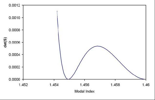Figure 1: The determinant of the system matrix vs. the modal index. Step index fiber with radius 2 μm, core index of 1.46, and a cladding of 1.45. The optical wavelength is 0.5 μm, and the order v = 0.

It is difficult to find the zero for curves of this type. The position of the zero is easily
passed over in the initial search for zero crossings. The shape of the curve in the
region of the zero is very nearly quadratic, so the best solution is to split the
determinant function into a product of two functions. In that case, the zeros can be
found by looking for zero crossings of the two functions separately. Suitable functions
can be found by considering the vector [A₀, C₀], as an eigenvector of S with
eigenvalue, equal to 0. The eigenvalues of S(n) are ,

Where T = S₁₁ + S₂₂. The determinant of a matrix is equal to the product of its
eigenvalues, so the product det(S(n)) = λ₁(n)λ₂(n) is a factoring convenient for
the zero finding task. A mode exists when either λ₁(n) = 0 or λ₂(n) = 0. The
advantage of searching for zeros of the two functions (23) is that the functions λ₁(n)
and λ₂(n) have zeros that are widely spaced apart, and are more easily found than
the zeros of the single determinant function.

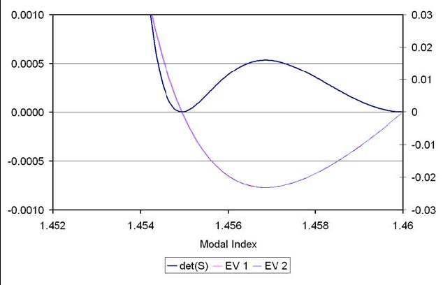Figure 2: Plot of the eigenvalues and determinant vs modal index.

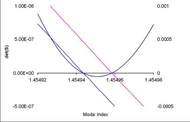Figure 3: Expanded view of the zero crossing region

LP Modes

Linearly Polarized modes can be found with the same style of approach as above, by
a transfer matrix analysis of multilayer fibers.In the LP analysis, the initial excitation is
assumed to have a linear polarization, and so a modal analysis supporting only one
field component is used. It can be shown this is a good approximation for fibers with
low refractive index contrast, as shown below.

Consider again the wave equation of (5), but this time use the vector identity (10)
directly on the electric wave equation instead of introducing the Debye potential. The
result is

From the Maxwell divergence equation (2)

so that

In the case of low index contrast waveguides, such as are found in most optical fibers,
the last term in (26) is negligible. The last term is the only one that contributes to
coupling among the field components of the electric field, so if this term is neglected,
the model will be a polarization preserving model. If the excitation was a linear
polarization parallel to the X axis, the model could be further simplified by considering
only the X component of (26). This shows that for the LP model, the governing
equation for the field is the Helmholtz equation (8) applied to the field component E_x.

The solution for LP modes is constructed in a similar way as for the vector modes.
The E_x is constructed in each layer as a linear combnation of Bessel functions (16)
and (17), except this time only two coefficients, A₁ and B₁, are required, since only
one function needs to be constructed. The physical consideration at the layer
boundaries is the continuity of E_x and its derivative. The two conditions are related
to the two coefficients A and B for each layer by 2×2 matrices. The modes are found
by setting up a calculation that assumes A₁ = 1 and B₁ = 0 for the first (inner
most) layer, and then calculating the coefficients in each subsequent layer by matrix
manipulations. The last layer has the condition that the coefficient ( A_M ) of the Bessel
function I_V must be zero, since this Bessel function is not bounded at infinity. This
last coefficient is a function of the order v and the modal index n, so the modes are
found by finding the zeros of A_M(n).

References

[1] K. Okamoto, Fundamentals of Optical Waveguides, (Academic Press, San Diego, 2000).

[2] C. Tsao, Optical Fibre Waveguide Analysis, (Oxford University Press, 1992), Part III

[3] C. Yeh and G. Lindgren, “Computing the propagation characteristics of radially stratified fibers: an efficient method”, Applied Optics 16(2) p483-493 (1977)
[4] J. Chilwell and I. Hodgkinson, “Thin-films field-transfer matrix theory of planar multilayer waveguides and reflection from prism-loaded waveguide”, Journal of the Optical Society of America A, 1 p742-753 (1984)