
Polarization mode dispersion
In ideal single-mode fibers, propagation constants of the two polarization Eigenmodes
are degenerate. In real telecommunications fibers, perturbations act on the fiber in a
way that it induces a birefringence, which splits this degeneracy. Consequently, when
a pulse is launched in a fiber, it gives rise to a differential group delay between the two
polarization Eigenmodes. The stochastic behavior of these perturbations is an issue
because it yields to the phenomenon of random mode coupling which makes
impossible the basic definition of the differential group delay.
Principal states of polarization
The Principal States of Polarization (PSP) model [Poole and Wagner, 1986[14]] is
based on the observation that at any given optical frequency, there exists a set of two
mutually orthogonal input states of polarization for which the corresponding output
states of polarization are independent of frequency to first order. The Differential
Group Delay (DGD) resulting from Polarization Mode Dispersion (PMD) is then
defined between the two output principal PSPs.
The birefringence in telecommunication single-mode fibers varies randomly along the
fiber length, an artifact of variation in the drawing and cabling process. Furthermore,
owing to the temperature dependence of many of the perturbations that act on the
fiber, the transmission properties typically vary with ambient temperature. In practice,
fluctuations in temperature strongly affect PMD time evolution. To evaluate properties
of long fiber spans, one adopts a statistical approach. In this case of long span fibers,
the polarization Eigenstates can only be defined locally and the birefringence vector
has to be considered as stochastic.
Dispersion vector definition
In the time domain, the Polarization Mode Dispersion (PMD) induces a time shift
between the two Principal States of Polarization (PSP).
In the frequency domain, the output state of polarization undergoes a rotation on the
Poincaré sphere about an axis connecting the two PSPs.
The rate and direction of rotation is given by the dispersion vector Ω(ω, z) given by:
![]()
where Pb – represents the negative output principal state.
The strength of the dispersion vector Ω(ω, z) is equal to the differential delay time Δτ
between the two output principal states, where its combined Stokes vector
corresponds to the Stokes vector of the negative output principal state. The direction
of the Dispersion Vector Ω defines an axis whose two intercepts with the surface of the Pointcaré sphere correspond to the two principal states of polarization at the fiber
output.
Poincaré sphere
The Poincaré sphere is a graphical tool that allows convenient description of polarized
signals and polarization transformations during propagation. A point within a unit
sphere can uniquely represent any state of polarization, where circular states of
polarization are located at the poles. The coordinates of a point within or on the
Poincaré sphere are the normalized Stokes parameters.
Ensemble simulation
Based on the Principal States of Polarization (PSP) model, one can model the whole
fiber as a sum of N trunks where each trunk represents a uniform and constant
birefringent device. A recursive formula describing the evolution of the dispersion
vector for N and N-1 concatenated trunks is the basis for the calculus of the first and
second order of the Differential Group Delay (DGD) induced by the Polarization Mode
Dispersion (PMD).
In the ensemble simulation model, the PMD calculation is repeated in a number of
runs. First, a set of concatenated fiber trunks is generated randomly. Then the
polarization mode dispersion is calculated. In the second run, a second set of trunks
is generated, followed by the PMD calculations. The process is repeated as many
times as it is required. Statistics of the PMD are calculated using the same number of
runs as the ensemble representation.
Spectral simulation
In the frequency domain, the Polarization Mode Dispersion (PMD) causes the state
of polarization at the output of a fiber to vary with frequency for a fixed input
polarization, which occurs in a cyclic fashion. When displayed on the Poincaré
sphere, the polarization at the output moves on a circle on the surface of the sphere
as the optical frequency is varied.
In the spectral simulation, a set of concatenated fiber trunks is generated randomly.
The calculations of polarization mode dispersion are performed over a range of
wavelengths.
First order dispersion definition
The Differential Group Delay (DGD) that is calculated based on a stochastic fiber
model (first order PMD) quantifies the first order Polarization Mode Dispersion.
This latter represents the discrete model for Polarization Mode Dispersion (PMD) and
is given by the following recursive formula [Bruyère, 1994[3]]
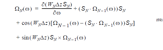
where
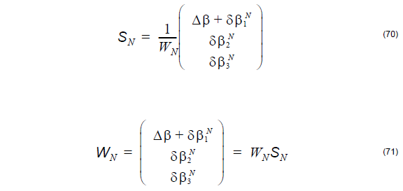
In the above, the symbol W with index N represents the birefringence of the fiber. It
consists of a background linear birefringence Δβ on top of which is added a
perturbation birefringence δβ. On the Poincaré sphere, the Δβ vector is
(Δβ, 0, 0) and the δβ vector is (δβ1, δβ2, δβ3), respectively. The above
recursive formula represents the discrete version of the Poole’s dynamical equation
[Poole et al., 1991[16]].
Mean value of the first order PMD
For a long fiber span, the average Differential Group Delay (DGD) has a square root
dependence on fiber length z as follows:

Root Mean Square (RMS) of the first order PMD
The root mean square differential delay time has also a square root of length
dependence:

The probability Density Function (PDF) of the differential delay time is Maxwellian:

Second order dispersion definition
The second order Polarization Mode Dispersion (second order PMD) is defined by the
following expression [Foschini and Poole, 1991[6]]:

where Ωω(ω, z) the first frequency derivative of the dispersion vector Ω:

The dispersion vector is defined in the section: Dispersion vector definition.
Effective Nonlinear Refractive Index
Usually one of the design goals when constructing a fiber is to minimize its
nonlinearities. The effective nonlinear coefficients of optical fibers depend on the
nonlinear indices of the bulk materials building the fiber and on its waveguiding
properties: shape of modes, degree of confinement, etc. As a result it can vary within
broad limits. OptiFiber calculates the eff. nonlinear coefficient as [Marcuse, 1991[8]]:
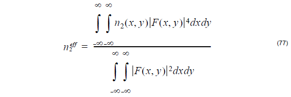
where n2(x, y) is the user-defined spatially dependent nonlinear refractive index of
the various fiber layers and F(x, y) is the normalized mode field pattern.
Interference (speckle) patterns (linear superposition/composition of modal fields)
With OptiFiber the user can calculate the superposition/interference pattern of an
arbitrary group of modes. Each of the modes has an arbitrary user defined guided
power and initial phase (a complex weighting coefficient assigned). This feature
targets applications such as coupling efficiency calculations, switching phenomena in
a few mode fiber sensors, etc.
Coupling efficiencies (linear decomposition of an input beam)
OptiFiber calculates the per-mode coupling efficiencies (the linear decomposition) of
a user defined input beam into an arbitrarily selected group of supported modes.
The decomposition coefficient is calculated using the following well-known
expression:
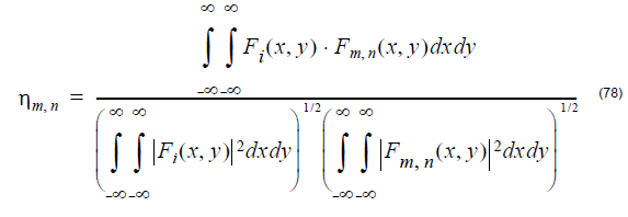
where Fi(x, y) is the input field, Fm. n(x, y) is the modal field.
Scanning
One of the most powerful features of OptiFiber software is the design optimization by
means of parameter scanning.“Scanning” is the name of the parametrical calculations
of some fiber characteristic versus certain technological properties or quantities of the
fiber design: for example the core/cladding refractive index difference, the spatial
width or some region, etc. It predicts automatically how any given fiber could be
optimized versus a design goal, for example small, but non-zero dispersion and
maximal mode area.
Compatibility with the NR-9200 Optical Fiber Analyzer from EXFO Inc.
Version 1.5 and later versions of OptiFiber are designed and developed to be fully
compatible with NR-9200 in the sense that it directly imports the ASCII files with the
experimental refractive index profile data, recorded by the low level drivers of the
device. It is as a software tool that supplements and extends the fiber characterization
capabilities of the NR-9200.
When the user chooses a NR-9200 Data File with a valid format the experimental data
is processed and the following parameters are extracted and imported in OptiFiber:
- Fiber Data: Fiber name, Fiber type, Cladding index
- Measurement Info: Operator, Date, Measurement wavelength, Comments
- Scanning details: Scan type, Data type, Number of points, Scan step, Data format
- The actual data
The input files may contain just one scan (X) or two scans (X and Y).
After that, the experimental data is processed and a single, axially symmetric profile
is formed from the available raw data.
The details of this process are controlled by the “Refractive index profile
preconditioning dialog” described in the “Dialog Boxes Reference”. It offers two
features:
- The ability to define the step (inversely proportional to the resolution) of the
numerical approximation of the refractive index. This is the minimal refractive index difference between two adjacent experimental points that are to be
considered belonging to different reference index regions in OptiFiber. It is
entered as a percentage of the maximal core-cladding difference. Lower values
mean finer approximation/more layers/longer computations and vice-versa. The
value of the step should be the best trade-off between accuracy and numerical
efficiency. - It offers the user the (optional) choice to reduce the ripples, imperfections and
spurious mechanical or optical noises of the data by means of low-pass Fourier
filtering and/or averaging. The bandwidth of the filter is given in percentage of the
highest frequency of the profile curve as a function of the point number. The
averaging substitutes every data point with the symmetrical mean value of the
respective number of adjacent points. When this is not possible (for example the
first point lacks left-standing neighboring points) the number of averaged points
is reduced accordingly. The recommended values of the filtering and averaging
parameters are 10 –15% and 2-3 respectively, however the overall quality of
smoothing depends also on the value of refractive index step (as described
above), so the user might prefer to fine-tune these three values for optimal results
in his particular case.
When the experimental data is imported, the user can proceed with defining other
parameters of the fiber, altering the profile data manually (for example by merging
some marginal layers of the cladding) and with running the various models currently
supported by OptiFiber.
The process of importing NR-9200 data is described in detail in “Tutorial
Lessons/Lesson 2”. See also the description of the “Menu/Import Profile” command
and of the “Refractive index profile preconditioning” dialog box.