
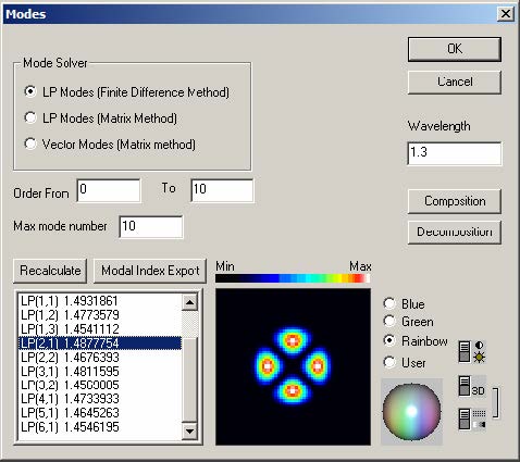
Modes dialog box
The “Modes” dialog box allows you to:
- Select the types of modes you are interested in
- Select the range of mode numbers you are interested in
- Find the spectrum of supported modes at the specified wavelength with their mode numbers and effective refractive indices
- Select a mode or group of modes for subsequent calculations.
- Preview the mode pattern of a selected mode in a number of ways.
- “Compose” a beam by the interference of an arbitrary group of supported modes.
- “Decompose” in input beam into an arbitrary group of supported modes (calculate input coupling efficiencies.)
To access this dialog box, do one of the following steps:
| Step | Action |
| 1 | Select “Modes” on the “Simulation” menu, or |
| 2 | Click the “Modes” icon in the “Navigator” pane |
 The elements and controls of “Modes” dialog box options are described below.
LP Modes (Finite Difference Method)
Check this option to calculate fiber propagation modes in the Linear Polarization (LP)
approximation (scalar modes). LP(m,n) modes are conventionally labeled using two
numbers: the azimuthal number m (the Order), and the radial number (mode number)
n. You can select the range of Order and the maximum n number for the solver.
LP Modes (Matrix Method)
This option finds LP modes as above, but by an exact method that uses radial transfer
matrices. See Appendix A – Fiber Mode Solvers by Matrix Method for details. This
method sometimes runs more slowly, especially if the profile has many layers.
However, the far field has the correct asymptotes, and this method is more accurate,
especially in the calculation of dispersion and other derivatives with wavelength.
Vectorial Modes
Check this option to calculate fiber propagation modes without the scalar
approximation. Conventionally, the vector modes have subsets of the hybrid HE and
EH modes, the Transverse Electric (TE) modes, and the Transverse Magnetic (TM)
modes. Hybrid (m,n) modes are conventionally labeled using the numbers: the
azimuthal number m (Order), and the radial number n. The vector modes are found
by a 4×4 transfer matrix method, see Appendix A – Fiber Mode Solvers by Matrix
Method for details.
Wavelength
This is the wavelength the calculated spectrum of modes relates to. It is independent
of the wavelength specified in the “Fiber Profile” dialog box.
Recalculate
Press the “Recalculate” button to start the mode solver.
List of modes
The results found by mode solver are displayed in the list of modes. The modes are
labeled according to the calculation option, with the modal index beside the label.
Modal Index Export
Export the contents of “List of modes” to a text file.
Mode field preview
Mode field can be previewed on the small display, where you can select the display
color mode and contrast.
Composition
Starts the “Composition” dialog box allowing to calculate arbitrary interference
combinations of the currently selected group of modes.
Decomposition
Starts the “Decomposition” dialog box allowing to calculate the coupling efficiencies
of an arbitrary input beam into each mode of the currently selected group of modes.
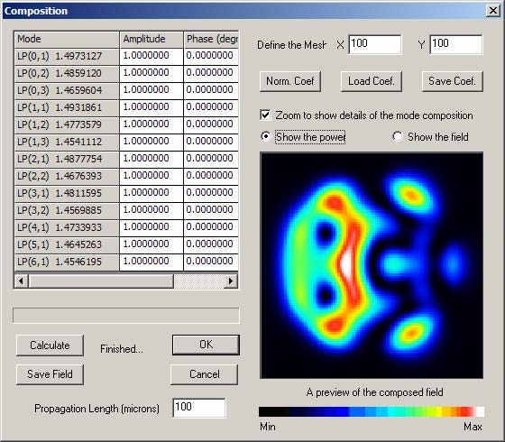
Composition dialog box
This dialog box controls the calculation of the superposition/interference pattern of an
arbitrary group of modes each of them having arbitrary power and input phase.
To use this feature, do the following steps:
| Step | Action |
| 1 | In the “Modes” dialog box, select a group of modes by using Ctrl-, Shift- and the left mouse button. |
| 2 | Press the “Composition” button. In the “Composition” dialog box, enter the weighting coefficient for each mode. |
| 3 | Press “OK” |
 The elements and controls of “Composition” dialog box options are described below.
Weighting coefficients table
Enter the complex coefficients assigned to each participating mode in the three-column
table (grid) in the upper left part of the dialog box
Preview display area
The graphical window in the lower right part of the dialog box shows a color-coded
topological view of the current pattern.
Calculate
Find the current interference pattern as defined by the set of modes and the
coefficients.
Define the Mesh
Increase/Decrease the resolution of the preview screen.
Norm Coef.
Normalizes the weighting coefficients. After normalization, the sum of the squared
magnitudes of all of the weighting coefficients is equal to 1.
Load Coef.
Load the weighting coefficients to a text file.
Save Coef.
Save the weighting coefficients to a text file.
Zoom
Check this option to zoom the details of the speckle pattern. Useful for fibers with
narrow core and wide cladding.
Power/Field
Display the intensity or the amplitude of the composed field.
Save field
Saves the calculated field to a text file. The saved file has the complex BCF3DCX 3D
file Format, described in the “Technical Background”.
Propagation Length
When this field is 0.0, the preview is the sum of the modes with amplitudes and
phases as indicated in the list. Enter a distance in microns in this field, and press
Calculate, to see the field as it would appear after a propagation of this distance.
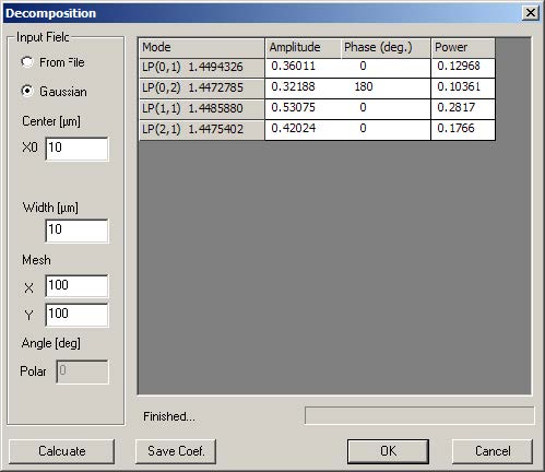
Linear decomposition of a given field distribution
This dialog box controls the calculation of the per-mode coupling efficiencies (the
linear decomposition) of an user defined input beam into an arbitrarily selected group
of supported modes.
To use this feature, do the following steps:
| Step | Action |
| 1 | In the “Modes” dialog box, select a group of modes by using Ctrl-, Shift- and the left mouse button. |
| 2 | Press the “Decomposition” button. In the “Decomposition” dialog box, define the parameters of the input beam. |
| 3 | Press “OK” |
 The elements and controls of “Decomposition” dialog box options are described
below.
Calculate
Find the decomposition coefficients for the current set of modes and the current input
beam.
Weighting coefficients table
Contains the calculated field (with their real and imaginary parts) and power
decomposition coefficients. The values in the “Power” are the squared sum of the real
and imaginary parts and have the meaning of the usual coupling coefficients.
From File
Read the input beam from a user defined file having the BCF3DCX complex 3D file
Format (please see the description in “Technical Background”).
Gaussian
The input beam is modeled as Gaussian field defined by the several parameters,
FWHM Width and polar angle.
Gaussian for Decomposition
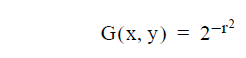 Where
Where
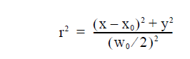
Center
The center position x0 of the input Gaussian beam.
Width
The width w0 of the input Gaussian beam.
Mesh
The number of point of the internal calculations. Higher value means better accuracy
of the coefficients at the expense of computating time.
Angle
Enter the polar angle between the input beam and the fiber axis.
Save Coef.
Export the coefficients to a text file.
Properties of Fundamental Mode dialog box
The “Properties of Fundamental Mode” dialog box controls the powerful parameter
scanning routines of OptiFiber related to the fundamental mode. It also allows the
user to select which characteristics of the fundamental mode to be calculated.
To access this dialog box, take one of the following steps:
| Step | Action |
| 1 | Select “Fundamental Mode” on the “Simulation” menu |
| 2 | Click the “Fundamental Mode” icon in the “Navigator” pane |
In the case of a simple step-index fiber it look as shown: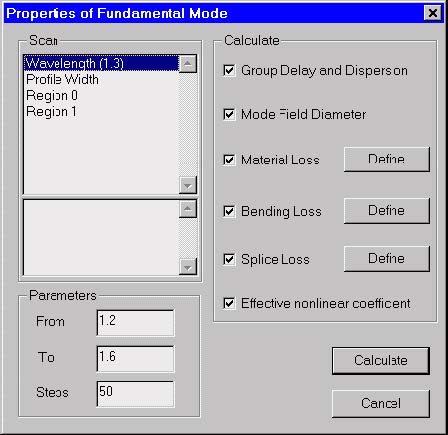 In order to use this dialog the user should have defined a legitimate profile in the
“Profile” dialog box.
The elements and controls of the “Properties of Fundamental Mode“ dialog box are
described below.
Scan
- The upper pane lists what is subjected to scanning:
- The wavelength within a spectral region.
- The profile as a whole within user-specified limits, for example
between 0.8 and 1.2 of the original width. This means that all spatial
dimensions of the original design are proportionally shrunk/expanded
at regular steps from 0.8L to 1.2L, where L is the initial width. - The single spatial regions of the profile.
- The lower pane lists the various technological parameters of the current region
that are available for scan calculations.
When “Wavelength” or “Profile Width” is selected in the upper pane, then there is no
other parameter to scan. When a region is selected, then all region parameters
available for scan calculations are displayed in the lower pane. Their number and
physical meaning depends on the type of the region. The available parameters may
include function parameters for function-defined regions. For example:
- If a simple “constant” region is selected, then for scanning are available:
- its spatial width and
- maximal refr. index
- If a “Gaussian function” region is selected, then for scanning are available:
- its spatial width
- maximal refr. index
- FWHM and
- central position
Parameters
The “Parameters” section refers to the range of parameter being scanned and the
number of steps. “From” – Initial value of the scan parameter “To” – Final value of the
scan parameter “Steps” – Number of calculation steps in the scan calculations
Calculate
The “Calculate” section allows you to select the fundamental mode characteristics to
be calculated versus the scan parameter.
The options are:
- Group Delay and Dispersion
- Mode Field Diameter
- Bending Loss
- Splice Loss
- Effective nonlinear coefficient
The Material Loss option always refers to scanning over the wavelength parameter.
You start the calculations by pressing the “Calculate” button.
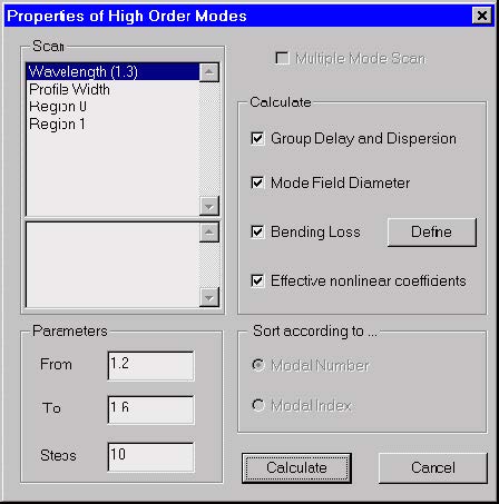
Properties of Higher Order Modes dialog box
The “Properties of Higher Order Modes” dialog box controls the powerful parameter
scanning routines of OptiFiber related to a higher order mode or a group of modes. It
also allows the user to select which modal characteristics to be calculated.
To access this dialog box, take the following steps:
| Step | Action |
| 1 | Select “Higher Order Modes” on the “Simulation” menu, or |
| 2 | Click the “Higher Order Modes” icon in the “Navigator” pane |
 In order to use this dialog the user should have:
- Defined a legitimate profile
- Solved for the spectrum of modes in the “Modes” dialog box and found that the
fiber is multi-mode at that wavelength. - Selected in the “Modes” dialog box
- a higher order mode, or
- a group of modes
If some of these conditions are not fulfilled, the user is automatically sent to the
respective place of OptiFiber to alter the design, to solve for modes, etc.
The logic of the scanning routines depends alternatively on the number of modes that
have been selected in the “Modes” dialog box. In the case of one selected higher
mode the “Properties of Higher Order Modes” works in the same way as the
“Properties of Fundamental Mode” dialog – it allows the defined characteristics of that
mode to be calculated versus some scanned parameter.
In the case of multiple selected modes the “Properties of Higher Order Modes”
calculates the defined characteristics of each mode. An option is offered to sort and
display the results:
- according the sequential number of the modes in the selected group.
- according the effective refr. index of the modes in descending order.
The elements and controls of “Properties of Higher Order Modes” are almost the
same as those of the “Properties of Fundamental Mode” dialog box and will not be
described separately.
Note: The calculations are performed for the mode or modes previously selected
in the “Modes” dialog box.
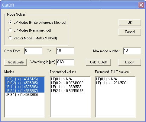
Cutoff dialog box
The “Cutoff” dialog box finds the spectrum of supported modes at a specified
wavelength, to select a set of the supported modes, and to find their cutoff
wavelengths. For explanation of the methods used to estimate the cutoffs, please
refer to the section “Cutoff Wavelengths” in the “Technical Background”.
To access this dialog box, take the following steps:
| Step | Action |
| 1 | Select “Cutoff” on the Simulation menu, or |
| 2 | Click the “Cutoff” icon in the “Navigator” pane |
| 3 | Enter wavelength and click Recalculate. |
 The elements and controls of the “Cutoff” dialog box are described below.
LP Modes (Finite Difference Method)
Check this option to calculate fiber propagation modes in the Linear Polarization (LP)
approximation (scalar modes). LP(m,n) modes are conventionally labeled using two
numbers: the azimuthal number m (the Order), and the radial number (mode number)
n. You can select the range of Order and the maximum n number for the solver.
LP Modes (Matrix Method)
This option finds LP modes as above, but by an exact method that uses radial transfer
matrices. See Appendix A – Fiber Mode Solvers by Matrix Method for details. This
method sometimes runs more slowly, especially if the profile has many layers.
However, the far field has the correct asymptotes, and this method is more accurate,
especially in the calculation of dispersion and other derivatives with wavelength.
Vectorial Modes
Check this option to calculate fiber propagation modes without the scalar
approximation. Conventionally, the vector modes have subsets of the hybrid HE and
EH modes, the Transverse Electric (TE) modes, and the Transverse Magnetic (TM)
modes. Hybrid (m,n) modes are conventionally labeled using the numbers: the
azimuthal number m (Order), and the radial number n. The vector modes are found by a 4×4 transfer matrix method, see Appendix A – Fiber Mode Solvers by Matrix
Method for details.
Wavelength
The wavelength at which the initial spectrum of modes is calculated. If the fiber is
single-mode at the specified wavelength – decrease it, in order to be able to select a
mode for the calculations.
Recalculate
Press the “Recalculate” button to start the mode solver.
List of modes
The results found by mode solver at the specified wavelength are here. The modes
are labeled according to the calculation option. The mode effective index of each
modes is given in parenthesis.
Lists of cutoff values
Displays the estimated cutoff wavelength values for the selected modes.
Two lists are available:
- “Theoretical values” and
- “Estimated ITU-T values”
in accordance with the two cutoff definitions. A cutoff wavelength is not defined for the
fundamental mode and therefore is marked ‘N/A’ (although occasionally, for quite inappropriate combination of parameters, the fundamental mode could be unsolvable for, a condition called “a numerical cutoff”).
Export
Click here to make an ascii text file that contains the modes listed in the columns
Theoretical values and Estimated ITU-T values.