
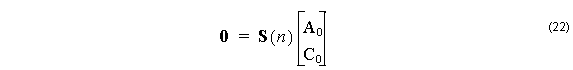
The matrix to describe the whole multilayer can be written as one 4×4 matrix, the product of all layers, one layer of which is shown in (21). The dispersion equation is usually constructed by setting the determinant of this 4×4 matrix product to 0, but this is not a good choice from the numerical point of view. In the limit of low index contrast, the modal indices can be very close to each other, making them hard to find by numerical methods, which tend to skip over closely spaced zeros. A more convenient condition comes from using rectangular matrices at the first and last layers, which are special cases. In the first layer, which contains r = 0, coefficients B0 and D0 must be zero, so the first matrix, D0 , is 4 x 2 consisting of the first and third columns of the D matrix in (20). Similarly, in the last layer, it is the coefficients AM and CM that must go to zero in (17), since those contain solutions Iν with unphysical growth. The last DM-1 will be of size 2 x 4, and consist of the first and third rows of D–1. The product of all these matrices will be of size 2×2, which we call S(n). (The dependence on n is written explicitly since it is the modal index to be found). A mode is obtained at a modal index n when a non-trivial solution is found to,
The condition det(S) = 0 is sufficient for a non-trivial solution. However this condition can be inconvenient for the case of certain modes of the low index contrast fiber. For example, consider a step index fiber with radius 2 μm , having a core index of 1.46 and a cladding of 1.45. For order zero ( ν = 0 ), the determinant of S will vary with the modal index n as shown in Figure 1.

Figure 1: The determinant of the system matrix vs. the modal index. Step index fiber with radius 2 μm , core index of 1.46, and a cladding of 1.45. The optical wavelength is 0.5 μm , and the order ν = 0 .
It is difficult to find the zero for curves of this type. The position of the zero is easily passed over in the initial search for zero crossings. The shape of the curve in the region of the zero is very nearly quadratic, so the best solution is to split the determinant function into a product of two functions. In that case, the zeros can be found by looking for zero crossings of the two functions separately. Suitable functions T can be found by considering the vector [ A0, C0 ], as an eigenvector of S with eigenvalue, λ equal to 0. The eigenvalues of S(n) are ,
![]()
Where T = S11 + S22 . The determinant of a matrix is equal to the product of its eigenvalues, so the product det( S( n ) ) =λ1 ( n )λ2 ( n ) is a factoring convenient for the zero finding task. A mode exists when either λ1 ( n ) = 0 or λ2 ( n ) = 0 . The advantage of searching for zeros of the two functions (23) is that the functions λ1 ( n ) and λ2 ( n ) have zeros that are widely spaced apart, and are more easily found than the zeros of the single determinant function.

Figure 2: Plot of the eigenvalues and determinant vs modal index.

Figure 3: Expanded view of the zero crossing region