
Modal analysis for optical waveguides is one of the most important area in modeling and simulation of guided wave photonic devices. The problem of the numerical boundary condition is expected to become much more accurate for the leaky modes, as the modal fields at the edges of the computation window are traveling waves and the modal leakage is extremely sensitive to the reflection from the artificial boundary. Since Perfectly Matched Layer (PML) boundary condition is applied to the modal analysis of optical waveguides it is possible to handle leaky modes. The PML will have no effects on the evanescent fields of the guided modes, but will attenuate the traveling field of the leaky modes. Thus, it is possible to simulate the leaky modes in a ARROW waveguide structure [5].
Vectoral Mode Calculation
By imposing ∂ ⁄ ∂z = 0 in Eq. (33), one can cast the Helmholtz equation into the following matrix form:
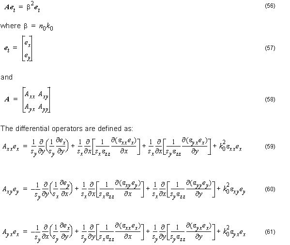

Equation 56 is a full-vectorial equation. The vectorial properties of the electromagnetic are include. Mxx ≠ Myy causes the polarization dependence. Mxy ≠ 0 and Myx ≠ 0 induces the polarization coupling between the two propagations. The discontinuities of the normal component of electric field at index interfaces, which is responsible for vectorial properties, have been considered in the formulation.
The FD method is used in the numerical solution of the vectorial wave equation, written in terms of the transverse components of the field. As a result, a conventional egeinvalue problems obtained without the presence of spurious modes, due to the implicit inclusion of the divergence conditions.
Equation 56 can be written as a conventional eigenvalue problem:
![]()
where β2 , I is the unit matrix and et is the eigenvector given by:
![]()
The transverse electric field components ex and ey , at any mesh point ( i, j ) are obtained from the eigenvector et for each propagating mode. In order to solve Equation 63, we use a solver that is based on Implicitly Restarted Arnold Method [10] available in MatLab Software and in a public domain library ARPACK. Using the Arnold Method, it is possible to solve large sparse problems by finding only selected eigenvalues which may be located in various parts of the spectrum. For instance, in waveguide problems one is typically interested in a few dominant modes which correspond to the eigenvalues with the largest real part. The most suitable technique for finding the dominant modes involves the shift-invert strategy in which eigenproblem Equation 13 is converted to the eigenproblem:

where σ is the shift. When an iterative solver is applied, the product of matrix operator and some varying vector x is repeatedly calculated. In the modified eigenproblem Equation 62, instead of calculating the inverse of matrix ( A – σI ) directly, a sparse LU decomposition of the matrix is performed.
Consequently, when y = ( A – σ I )–1 x product is required, a linear system of equations
( A – σI )y = x is solved instead. The convergence rate in the shift-invert mode in iterative method depends on the shift σ . In the waveguide analysis it is convenient to choose the shift so that σ = εmax .
In this case, the dominant modes correspond to the eigenvalues of Equation 65 possessing the largest magnitude.