
E-Formulation: The vector wave equation for the electric fields
![]()
On the transverse plane Equation (19) becomes:
![]()
The solution of the wave equation Equation 31 can be separated as a slowly varying envelope and a fast-oscillating phase term:
![]()
Using Gauss’ Law, ![]() we get:
we get:

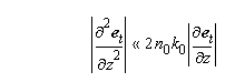
If the refractive index varies slowly along the propagation direction , which is valid for must photonic guided-wave devices. Then the mentioned term above is much smaller than the other ones in Equation 33. Thus one can derive:
![]()
Therefore,

If the transverse components of an electromagnetic field are known, longitudinal component may be readily obtained by application of the zero divergence constraint
![]() (Gauss’ Law).
(Gauss’ Law).
Therefore, the transverse components are sufficient to describe the full-vectorial
natures of the electromagnetic field.
Finally by using equations Equation 35 and Equation 32 into wave equation
Equation 31, we can write the following wave equation in terms of the transverse
components of electric field.
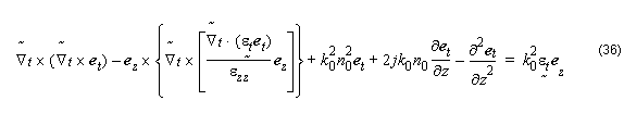
Note: The elimination of the axial component using the divergence condition, ∇ ⋅ D = 0 , guarantees the complete elimination of spurious modes. In addition using just two components instead of three reduces computational efforts and resource usage.
We can write Equation 36 in a operator form:
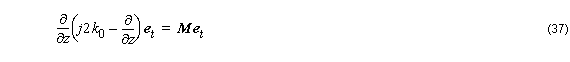
where the operator is defined as
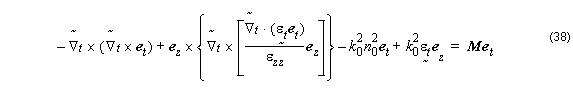
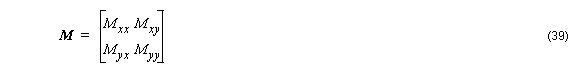
Matrix M can also be written in component:
Differential operators definition:
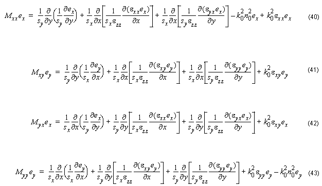
Equation 37 is a full-vectorial equation. The vectorial properties of the electromagnetic are included. Mxx ≠ Myy causes the polarization dependence. Mxx ≠ 0 and Myy ≠ 0 induces the polarization coupling between the two polarizations. The discontinuities of the normal component of electric field at index interfaces, which is responsible for the vectorial properties, have been considered in the formulations. The discrete form of the differential operators in the governing equations (Equation 40 – Equation 43) may be found in a straightforward way [8]. At the index discontinuities, although the normal electric field are not continuous, the displacement vectors Dx are continuous across the index interfaces along the x – and y – axis, respectively. Therefore, the central difference scheme can be applied directly. The 126 operator M does not change its sparsity with the introduction of the PML, except that the matrix elements are modified according to the discretization of the transverse operator in the PML region [7].
Wide Angle FD-VBPM
In paraxial formulation we make use of the slowly varying envelope approximation:
The use of the paraxial approximation limits the method to structures where the beam propagates in directions that makes a small angle with respect to the axis of propagation. Wide angle BPM circumvents that restriction of the paraxial approximation by retaining the second derivative of the envelope along z . Therefore it is not necessary to have the phase variation along z almost constant and uniform over the cross section. Neither is it required for field amplitude to change slowly along z . This allows the simulation of multiple propagating modes traveling a widely different off-axis angles, and there is no need to accurately guess the “reference” index n0 . Here we refer to the angle relative to the z -axis as an off-axis angle [7].
Equating operators on et on the left and right sides of the Equation 37 gives the recursion [8]:
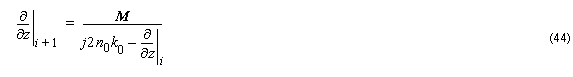
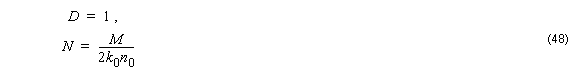
which generates successively better approximations to the actual ∂ ⁄ ∂z . We refer to this as a Pade recursion. It turns out that if the recursion is started assuming ∂ ⁄ ∂z ]0 = 0 , then the first recursion yields paraxial BPM. Therefore one can get
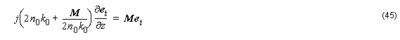
for a paraxial propagator.
Equation 45 is capable of describing the propagation of continuous vectorial electromagnetic waves in linear, isotropic, and inhomogeneous medias.
The solution to Equation 45 can be written in a exponential form:
![]()
which can also be approximated by a weighted finite difference form:
![]()
Here Δ z is the longitudinal step size, α is a weighting factor which controls the finite-difference scheme. For instance, α = 1 , corresponds to the standard implicit scheme and
α = 0 is explicit ; the Crank-Nicholson scheme corresponds to α = 0.5 . The choice of α affects the stability, the numerical dissipation, and the numerical dispersion of the scheme. Applying the Von Neumann Analysis, it is possible to prove that the weighted finite-difference scheme is unconditionally stable for α ≥ 0.5 , which means that the stability criteria is independent of both longitudinal step size and transverse mesh sizes [7].
We get.
for paraxial.
Using Pade recursion we get:
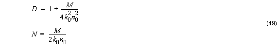
for wide angle-Pade(1,1).
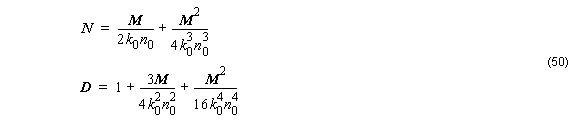
for wide angle-Pade(2, 2).
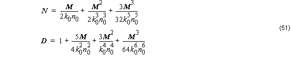
for wide angle-Pade(3, 3), and
for wide angle-Pade(4, 4).
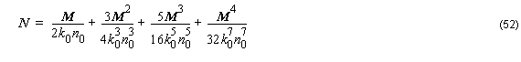
As can been seen, successive recursions yield operator expressions of increasing algebraic complexity, all of which can be reduced to a rational polynomial:

Applying this operator to et and discretizing:

In order to solve Equation 54 we use the multistep method developed by Hadley [8]. The advantage of the multistep method is that the matrix equation to be solved in each step is the same size as the Fresnel equation.
We can recast Equation 47 in the following form:
![]()
where { et }l and { et }l + l are field vectors at two sequential steps l and l + 1 , A and B are nonsymmetric complex band matrices.
The system in Equation 52 is solved efficiently by the well established sparse matrix solver BiConjugate Gradients Stabilized method (bicgstab) [9].